光线追踪技术是计算机图形学的一类全局光照算法,目前的影视行业大多都采用光线追踪做离线渲染。本章开始构建一个光线追踪离线渲染器(路径追踪),深入理解光线追踪的技术原理。主要参考资料为Peter Shirley的《Ray Tracing in One Weekend》。数学库沿用之前自己写的3D数学库,这方面的东西不再赘述。相关的完全代码在这里 。
一、光线追踪纵览 光线追踪 (Ray Tracing) 算法是一种基于真实光路模拟的计算机三维图形渲染算法,相比其它大部分渲染算法,光线追踪算法可以提供更为真实的光影效果。此算法由 Appel 在 1968 年初步提出,1980 年由Whitted 改良为递归算法并提出全局光照模型。直到今天,光线追踪算法仍是图形学的热点,大量的改进在不断涌现。基于对自然界光路的研究, 光线追踪采取逆向计算光路来还原真实颜色。追踪的过程中涵盖了光的反射、折射、吸收等特性 (精确计算), 并辅以其它重要渲染思想 (进一步模拟)。 其中包含了重要方法,诸如冯氏光照模型 (Phong Shading)、辐射度(Radiosity)、光子映射 (Photon Mapping)、蒙特卡罗方法 (Monte Carlo) 等等。鉴于光线追踪算法对场景仿真程度之高,其被普遍认为是计算机图形学的核心内容, 以及游戏设计、电影特效等相关领域的未来方向。 近年来由于硬件系统的迅速改良, 基于分布式、GPU, 甚至实时渲染的光线追踪显卡也纷纷出现(本人就是入手了一块实时光追显卡rtx2070)。
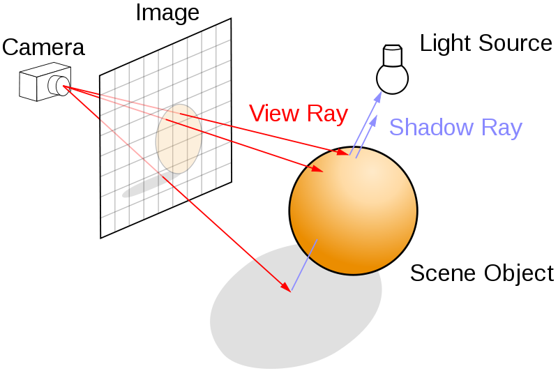
光线追踪算法是一种非常自然的技术,相比于光栅化的方法,它更加简单、暴力、真实。与光栅化根据物体计算所在的像素的方式不同,光线路径追踪的方法是一个相反的过程,它在于用眼睛去看世界而不是世界如何到达眼中。如下图所示,从视点出发向屏幕上每一个像素发出一条光线View Ray,追踪此光路并计算其逆向光线的方向,映射到对应的像素上。通过计算光路上颜色衰减和叠加,即可基本确定每一个像素的颜色。
图1 光线追踪示意图 可以看到光线追踪是一个递归的过程。发射一束光线到场景,求出光线和几何图形间最近的交点,如果该交点的材质是反射性或折射性的,可以在该交点向反射方向或折射方向继续追踪,如此递归下去,直到设定的最大递归深度或者射线追踪到光源处(或者背景色),如此便计算处一个像素的着色值。
基本的光线追踪tracing()递归算法如下所示:
Algorithm 1: 光线追踪递归算法
Input: 射线ray
Output: 反向光颜色
Function tracing():
if no intersection with any object then return background color else obj $\leftarrow$ find nearest object from the ray; reflect ray $\leftarrow$getReflectRay(obj); refract ray $\leftarrow$ getRefractRay(obj); main color $\leftarrow$ the radiance of obj; reflect color $\leftarrow$ tracing(reflect ray); refract color $\leftarrow$ tracing(refract ray);
return mix(main color, reflect color, refract color);
二、实现光线追踪渲染器 采用C++语言不借助第三方图形渲染API实现一个简易的光线追踪器,为了将最后的结果显示出来,我采用stb_image 将计算得到的像素矩阵保存为png图片。本篇实现的光线追踪只包含求交运行、计算光线反射和折射向量、反走样、景深等较为初级的方面,而实现的材质包含磨砂材质、玻璃材质和金属材质。
1、摄像机 与光栅化的空间变换过程相反,光线追踪大部分操作都是在世界空间中进行,因而需要将屏幕空间的像素坐标变换到世界空间中,并相应地发射出一条射线。在这里我们不再构建矩阵,直接求解出摄像机的三个坐标轴,然后根据视锥体的视域fov和屏幕的宽高比aspect得到每个像素发射出来的射线。
首先我们创建一个射线类$Ray$,射线通常用一个射线原点$m_origin$和射线方向$m_direction$表示,射线上的每个点则表示为$p(t)=m_origin+t*m_direction$,射线上每一个独立的点都有一个自己唯一的$t$值。因而创建的$Ray$类如下所示,其中$pointAt$函数根据给定的$t$值返回相应的射线上的点:
1
2
3
4
5
6
7
8
9
10
11
12
13
14
15
16
17
18
19
20
21
22
class Ray { private : Vector3D m_origin; Vector3D m_direction; public : Ray() = default ; ~Ray() = default ; Ray(const Vector3D &org, const Vector3D &dir) :m_origin(org), m_direction(dir) { m_direction.normalize(); } Vector3D getOrigin () const { return m_origin; } Vector3D getDirection () const { return m_direction; } Vector3D pointAt (const float &t) const { return m_origin + m_direction * t; } };
我们实现的基于cpu的光线追踪核心渲染流程是对给定分辨率的像素矩阵,逐行逐列地遍历每个像素坐标,如下所示:
1
2
3
4
5
6
7
8
9
10
11
unsigned char *RayTracing::render(){ for (int row = 0 ;row < m_height;++ row) { for (int col = 0 ;col < m_width;++ col) { ...... } } return m_image; }
因而对于每个给定的像素坐标$(x,y)$,我们需要获取这个像素坐标对应的发射出去的射线,首先我们把值域为$[0,m_width]$和$[0,m_height]$的像素坐标映射到$[0,1]$,正如如下所示:
1
2
float u = static_cast <float >(col) / static_cast <float >(m_config.m_width);float v = static_cast <float >(row) / static_cast <float >(m_config.m_height);
接下来我们根据$u$和$v$获取射线方向向量,这涉及到两个方面,一个摄像机的坐标系统,另一个是关于视锥的大小设置。摄像机的坐标轴决定了当前的朝向,视锥的大小设定决定了当前视域的大小。为此,我把摄像机与视锥合并一起,坐标系类型依然是右手坐标系。创建的摄像机类如下所示:
1
2
3
4
5
6
7
8
9
10
11
12
13
14
15
16
17
18
19
20
21
22
23
24
25
26
27
28
29
30
31
class Camera { public : Vector3D m_pos; Vector3D m_target; Vector3D m_lowerLeftCorner; Vector3D m_horizontal; Vector3D m_vertical; float m_fovy, m_aspect; Vector3D m_axisX, m_axisY, m_axisZ; Camera(const Vector3D &cameraPos, const Vector3D &target,float vfov, float aspect); Ray getRay (const float &s, const float &t) const ; Vector3D getPosition () const { return m_pos; } Vector3D getTarget () const { return m_target; } Vector3D getAxisX () const { return m_axisX; } Vector3D getAxisY () const { return m_axisY; } Vector3D getAxisZ () const { return m_axisZ; } void setPosition (const Vector3D &pos) void setTarget (const Vector3D &_tar) void setFovy (const float &fov) void setAspect (const float &asp) private : void update () };
其中$m_pos$即摄像机的世界坐标位置,$m_target$即目标位置,而$m_lowerLeftCorner$表示视锥近平面的左下角位置,$m_horizontal$表示近平面在摄像机坐标系下水平方向的跨度,$m_vertical$则是近平面在摄像机坐标系下垂直方向的跨度。$m_fovy$和$m_aspect$分别是视锥的垂直视域和屏幕的宽高比。初始时我们传入摄像机坐标、目标点以及垂直视域和视口宽高比,然后我们根据这些计算摄像机的三个坐标轴,以及近平面的位置:
1
2
3
4
5
6
7
8
9
10
11
12
13
14
15
16
17
18
19
20
21
void Camera::update(){ const Vector3D worldUp (0.0f , 1.0f , 0.0f ) float theta = radians(m_fovy); float half_height = static_cast <float >(tan (theta * 0.5f )); float half_width = m_aspect * half_height; m_axisZ = m_pos - m_target; m_axisZ.normalize(); m_axisX = worldUp.crossProduct(m_axisZ); m_axisX.normalize(); m_axisY = m_axisZ.crossProduct(m_axisX); m_axisY.normalize(); m_lowerLeftCorner = m_pos - m_axisX * half_width - m_axisY * half_height - m_axisZ; m_horizontal = m_axisX * 2.0f * half_width; m_vertical = m_axisY * 2.0f * half_height; }
然后我们对于给定在$[0,1]$的$u$和$v$,就可以计算出一条对应的射线向量了。
1
2
3
4
Ray Camera::getRay(const float &s, const float &t) const { return Ray(m_pos , m_lowerLeftCorner + m_horizontal * s + m_vertical * t - m_pos ); }
1
2
3
4
5
6
7
8
9
10
for (int row = m_config.m_height - 1 ; row >= 0 ; --row){ for (int col = 0 ; col < m_config.m_width; ++col) { float u = static_cast <float >(col + drand48()) / static_cast <float >(m_config.m_width); float v = static_cast <float >(row + drand48()) / static_cast <float >(m_config.m_height); Ray ray = camera.getRay(u, v); ...... } }
2、物体求交 射线发射出去之后要与物体进行求交运行,对于这类能够被射线碰撞到的物体我们把它抽象为$Hitable$,并用一个虚函数$Hit$作为所有的碰撞求交的接口,创建$Hitable$虚类如下:
1
2
3
4
5
6
7
8
9
10
11
12
13
14
15
16
class Material ;struct HitRecord { float m_t ; Vector3D m_position; Vector3D m_normal; Material *m_material; }; class Hitable { public : Hitable() = default ; virtual ~Hitable() {} virtual bool hit (const Ray &ray, const float &t_min, const float &t_max, HitRecord &ret) const 0 ; };
可以看到我们还创建了一个$HitRecord$结构体,它包含一次射线碰撞求交的结果记录,其中$m_t$是射线方程的参数$t$,$m_position$是交点的位置,$m_normal$是交点的法向量,而$m_material$则是交点所在物体的材质,求交之后我们需要根据这些记录来计算物体的折射、反射。
$Hitable$中的$hit$接口以一条射线$ray$作为输入参数,以一个$Hitable$的引用$ret$作为求交的结果记录,函数返回布尔值以表示是否发生了射线碰撞。此外,值得一提的是我们还输入了两个参数,分别是$t_min$和$t_max$,这个是我们自己对射线线段长度做的一个限制,可以分别去掉太近和太远的物体。
然后我们需要向场景中添加物体,光线追踪器的一个”Hello, world!”是球体。我们知道,一个球体的数学表达式为如下所示:
其中$c=(cx,cy,cz)$是球体的球心,$R$为球体半径。我们现在要求的就是,对于射线上的一点$P(t)=S+tV$,使得$(x,y,z)=P(t)=S+tV$带入公式$(1)$成立,公式$(1)$可以写成点乘的形式如下:
将$P=P(t)=S+tV$带入公式$(2)$可得:
可以看到公式$(3)$中只有$t$未知,它是一个一元二次方程。对于任意的一元二次方程$at^2+bt+c=0$,其解有如下形式:
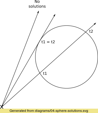
其中根号内的$D=b^2-4ac$称为根的判别式,它可以反应多项式根的数量。若$D>0$则有两个实数根,若$D=0$则只有一个实数根,若$D<0$则没有实数根。我们首先可以根据判别式判断是否存在交点,然后再求出具体的交点坐标。下面的$Hit$函数,我们首先求出多项式方程的常数项$a$、$b$和$c$,然后求判别式,最后再有解的情况下求取交点。注意,在有两个交点的情况下,我们首先取较近的点,不符合再取较远的那个点。只有一个交点的情况下(如下图2所示),我们不当作射线发生了碰撞(擦边而过)。
1
2
3
4
5
6
7
8
9
10
11
12
13
14
15
16
17
18
19
20
21
22
23
24
25
26
27
28
29
30
31
32
33
34
35
36
37
38
39
40
41
42
43
44
45
class Sphere :public Hitable { public : float m_radius; Vector3D m_center; Material *m_material; Sphere(const Vector3D &cen, const float r, Material *mat) :m_center(cen), m_radius(r), m_material(mat) {} ~Sphere() { if (m_material)delete m_material; m_material = nullptr ; }; virtual bool hit (const Ray &ray, const float &t_min, const float &t_max, HitRecord &ret) const }; bool Sphere::hit(const Ray &ray, const float &t_min, const float &t_max, HitRecord &ret) const { Vector3D oc = ray.getOrigin() - m_center; float a = ray.getDirection().dotProduct(ray.getDirection()); float b = oc.dotProduct(ray.getDirection()); float c = oc.dotProduct(oc) - m_radius * m_radius; float discriminant = b * b - a * c; if (discriminant > 0 ) { float temp = (-b - sqrt (b * b - a * c)) / a; if (temp > t_min && temp < t_max) { ret.m_t = temp; ret.m_position = ray.pointAt(ret.m_t ); ret.m_normal = (ret.m_position - m_center) / m_radius; ret.m_material = m_material; return true ; } temp = (-b + sqrt (b * b - a * c)) / a; if (temp > t_min && temp < t_max) { ret.m_t = temp; ret.m_position = ray.pointAt(ret.m_t ); ret.m_normal = (ret.m_position - m_center) / m_radius; ret.m_material = m_material; return true ; } } return false ; }
图2 射线与球体的相交情况 当场景中有多个物体时,当前的做法是在每次求交时遍历所有的物体,我们需要一个$HitableList$来存储这些物体。我们令$HitableList$继承自$Hitable$,这样$HitableList$就表现得好像只有一个很大的物体一样,并在实现$hit$函数中对场景得所有物体遍历调用他们的$Hit$方法:
1
2
3
4
5
6
7
8
9
10
11
12
13
14
15
16
17
18
19
20
21
22
23
24
25
26
27
28
29
30
31
32
33
34
35
36
37
38
class HitableList :public Hitable{ public : std ::vector <Hitable*> m_list; HitableList() = default ; ~HitableList() = default ; void addHitable (Hitable *target) void clearHitable () { for (int x = 0 ; x < m_list.size(); ++x) { delete m_list[x]; m_list[x] = nullptr ; } } virtual bool hit (const Ray &ray, const float &t_min, const float &t_max, HitRecord &ret) const }; bool HitableList::hit(const Ray &ray, const float &t_min, const float &t_max, HitRecord &ret) const { HitRecord tempRec; bool hitAny = false ; double closestSoFar = t_max; for (unsigned int x = 0 ; x < m_list.size(); ++x) { if (m_list[x]->hit(ray, t_min, closestSoFar, tempRec)) { hitAny = true ; closestSoFar = tempRec.m_t ; ret = tempRec; } } return hitAny; }
此外,值得一提的是,在$HitableList$的$hit$函数中我们需要做一个类似于深度测试的步骤,我们从摄像机发射的射线只能跟最靠近摄像机的那个交点做反射、折射,一条射线发射出去可能会与多个物体相交,我们必须取最近的交点。这个距离我们用射线方程中的$t$来描述,显然$t$越大则交点越远,因此用$closestSoFar$来记录当前获取的交点的最小$t$,以此作为$t$的上限,这样最终求出来的必然就是最近的交点。
3、物体材质 现在我们的一个问题就是求出交点之后,光线在交点上做什么样的反射和折射?这取决于物体的材质。若物体的材质是透明的玻璃,那么光线一般做折射;而若物体是光滑的镜面,则光线做完美的反射。针对不同物体的材质,光线的散射情况各不相同,为此我们创建一个虚类$Material$,并把光线散射的这一过程抽象为$sactter$函数接口。
1
2
3
4
5
6
7
8
9
class Material { public : Material() = default ; virtual ~Material() = default ; virtual bool scatter (const Ray &in, const HitRecord &rec, Vector3D &attenuation, Ray &scattered) const 0 ;};
可以看到,$scatter$函数接收入射射线$Ray$以及求交获得的$HitRecord$,计算散射光线的向量,返回的结果表示是否发生了散射。其中的$attenuation$本质上是物体自身的反射颜色,之所以叫$attenuation$是因为光线照射到物体上,物体一般会吸收光线中的大部分颜色,然后仅反射自身颜色的部分,这个过程使得光线在反射过程中不断衰减。
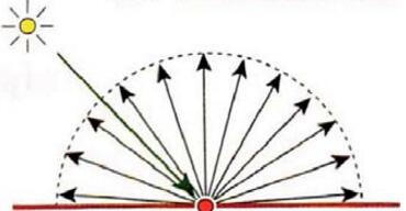
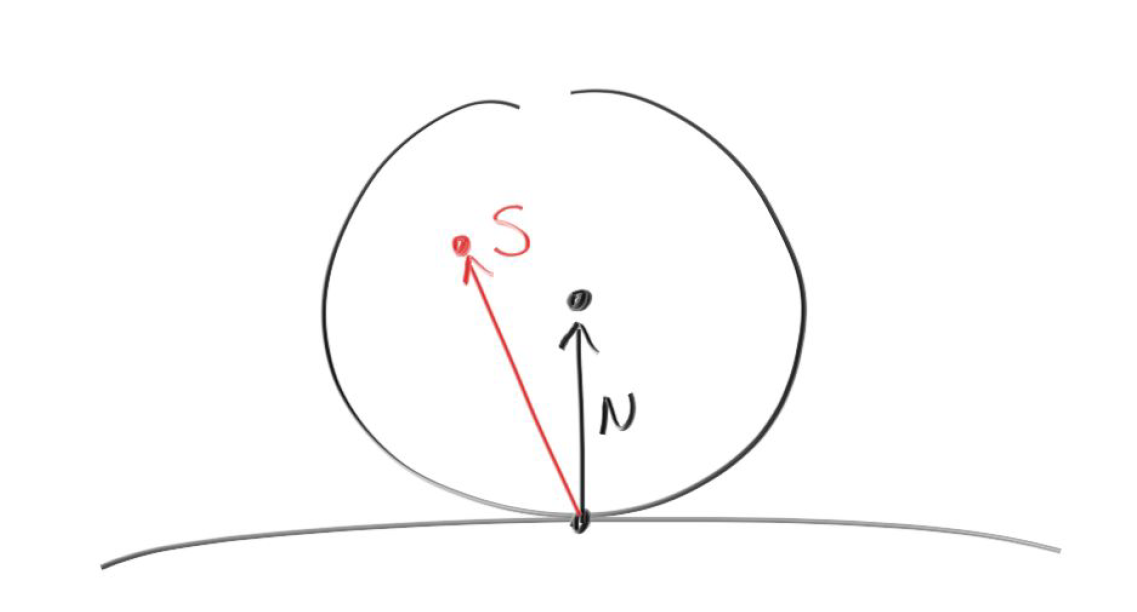
3.1 Lambertian反射材质 首先我们要实现的是Lambertian反射的材质,Lambertian反射也叫理想散射。Lambertian表面是指在一个固定的照明分布下从所有的视场方向上观测都具有相同亮度的表面,Lambertian表面不吸收任何入射光。Lambertian反射也叫散光反射,不管照明分布如何,Lambertian表面在所有的表面方向上接收并发散所有的入射照明,结果是每一个方向上都能看到相同数量的能量。这是一种理想情况,现实中不存在完全漫反射,但Lambertian可以用来近似的模拟一些粗糙表面的效果,比如纸张。
图3 Lambertian反射 为了实现Lambertian表面的均匀反射现象,我们令射线碰撞到表面之后,在交点的半球方向上随机地反射,只要随机性够均匀,我们就能模拟出理想散射的情况。为此,我们取一个正切于交点$P$表面的单位球体,在这个球体内随机取一个点$S$,则反射的向量就为$S-P$。这个正切于交点$P$表面的单位球体不难求得,设交点$P$的单位法向量为$N$,那么该正切球体的球心为$P+N$。我们首先在球心为原点的单位球内随机求得一个方向向量,然后将这个方向向量加上正切球体的球心即可得出反射的方向向量。($drand48$是生成$[0,1)$之间的均匀随机数函数,一般linux下才有这个内建函数,windows下没有,所以我们就自己写了。)
1 2 3 4 5 6 7 8 9 10 11 12 13 14 15 16 17 18 19 20 21 22 23 24 25 26 27 28 29 30 31 32 33 34 35 36 37 38 39 40 41 42 43 44 45 #define rndm 0x100000000LL #define rndc 0xB16 #define rnda 0x5DEECE66DLL static unsigned long long seed = 1 ; inline double drand48 (void ) { seed = (rnda * seed + rndc) & 0xFFFFFFFFFFFF LL; unsigned int x = seed >> 16 ; return ((double )x / (double )rndm); } =============================================================== static Vector3D randomInUnitSphere() { Vector3D pos; do { pos = Vector3D(drand48(), drand48(), drand48()) * 2.0f - Vector3D(1.0 , 1.0 , 1.0 ); } while (pos.getSquaredLength() >= 1.0 ); return pos; } =============================================================== class Lambertian : public Material { private : Vector3D m_albedo; public : Lambertian(const Vector3D &a) : m_albedo(a) {} virtual ~Lambertian() = default ; virtual bool scatter (const Ray &in, const HitRecord &rec, Vector3D &attenuation, Ray &scattered) const }; bool Lambertian::scatter(const Ray &in, const HitRecord &rec, Vector3D &attenuation, Ray &scattered) const { Vector3D target = rec.m_position + rec.m_normal + Vector3D::randomInUnitSphere(); scattered = Ray(rec.m_position, target - rec.m_position); attenuation = m_albedo; return true ; }
其中的$m_albedo$为物体自身的反射颜色。
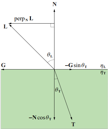
3.2 金属镜面反射材质 金属的表面比较光滑,因而不会呈现出光线随机散射的情况。对于一个完美镜面的材质来说,入射光线和反射光线遵循反射定律,即光射到镜面上时,反射线跟入射线和法线在同一平面内,反射线和入射线分居法线两侧,并且与界面法线的夹角(分别叫做入射角和反射角)相等。反射角等于入射角。
求反射向量如下图4所示,比较简单,不再赘述。
图4 反射向量
1
2
3
4
static Vector3D reflect (const Vector3D &ray, const Vector3D &normal) return ray - normal * (ray.dotProduct(normal)) * 2.0f ; }
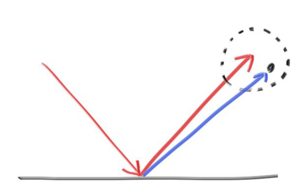
对于一个完美镜面的金属材质来说,我们只需求出反射向量,然后按照这个反射向量递归下去就行了。但是有些金属并没有那么光滑,它的高光反射并没有那么锐利,为此我们对求出的反射向量做一定的扰动,使反射向量在一定的波瓣内随机,这个波瓣有多大由用户决定(波瓣越大则金属越粗糙)。废话不多说直接上图就明白了。
我们在反射向量的终点上取一个给定半径的球体,在这个球体内随机选一个点作为新的反射向量的终点即可。这个半径的大小我们用$m_fuzz$变量存储,交给用户决定。
1
2
3
4
5
6
7
8
9
10
11
12
13
14
15
16
17
18
19
20
21
22
class Metal :public Material{ private : float m_fuzz; Vector3D m_albedo; public : Metal(const Vector3D &a, const float &f) : m_albedo(a), m_fuzz(f) { if (f > 1.0f )m_fuzz = 1.0f ; } virtual ~Metal() = default ; virtual bool scatter (const Ray &in, const HitRecord &rec, Vector3D &attenuation, Ray &scattered) const }; bool Metal::scatter(const Ray &in, const HitRecord &rec, Vector3D &attenuation, Ray &scattered) const { Vector3D reflectedDir = Vector3D::reflect(in.getDirection(), rec.m_normal); scattered = Ray(rec.m_position, reflectedDir + Vector3D::randomInUnitSphere() * m_fuzz); attenuation = m_albedo; return (scattered.getDirection().dotProduct(rec.m_normal) > 0.0f ); }
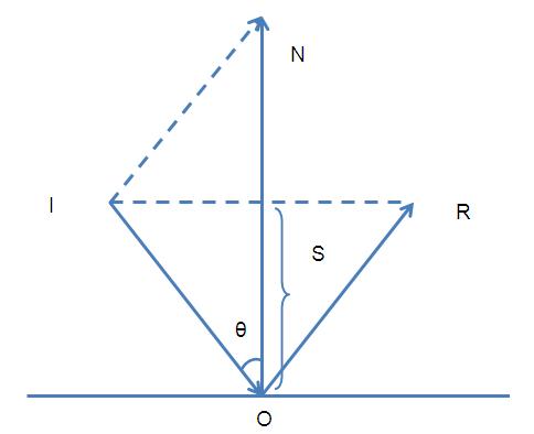
3.3 透明玻璃折射材质 对于水、玻璃和钻石等等物体的材质,光线照射到它们的表面时,它会把光线分成折射(也叫透射)光线和反射光线两部分。我们实现的材质采用随机的策略, 就是在折射和反射两个部分中随机选取一种。首先我们要根据入射向量、法线以及入射介质系数和折射介质系数计算折射方向向量,相比反射向量,推导计算的过程稍微有点复杂。折射表面有折射系数属性,根据Snell定律,如图5所示,入射角$\theta _L$和折射角$\theta _T$之间的关系有:
图5 折射向量的计算 其中,$\eta _L$时光线离开的介质的折射系数,$\eta _r$是光线进入的介质的折射系数。空气的折射系数通常定位$1.00$,折射系数越大,则在两种不同介质之间光线弯曲效果越明显。$N$和$L$都是单位方向向量。折射向量$T$可为与法向量平行的向量$-Ncos\theta_T$和垂直的向量$-Gsin\theta _T$,$G$是上图所示的单位向量。而$perp_NL$与$G$向量平行,且$||perp_NL=sin\theta_L||$,故有:
折射向量$T$可以表示为:
利用公式$(6)$,我们可以将上式中的正弦商替换为$\eta _L/\eta _T$,可得:
注意到公式$(9)$中的$cos\theta_T$未知,用$\sqrt{1-sin^2\theta_T}$替换$cos\theta_T$,再用$(\eta_L/\eta_r)sin\theta_L$代替$sin\theta_T$,可得:
最后再用$1-cos^2\theta_L=1-(N\cdot L)^2$代替$sin^2\theta_L$,得到最终的表达式为:
如果$\eta_L>\eta_T$,则上式平方根里的数值可能为负,这种情况发生在当光线从一个大折射率的介质进入一个小折射率的介质时,此时光线与表面之间的入射角较大。特别的,若仅当$sin\theta_L\leq \eta_r/\eta_L$时,公式$(11)$有效,如果平方根里的数值为负,则会出现所谓的全内反射现象,也就是光线不被折射,仅在介质内部反射。此外,需要注意的是,我们在程序实现中的入射向量与图5中$L$是相反的,所以需要将公式中的$(11)$的入射向量取反,如下所示:
1
2
3
4
5
6
7
8
9
10
11
12
13
14
15
static bool refract (const Vector3D &ray, const Vector3D &normal, float niOvernt, Vector3D &refracted) Vector3D uv = ray; uv.normalize(); float dt = uv.dotProduct(normal); float discriminant = 1.0f - niOvernt * niOvernt * (1.0f - dt * dt); if (discriminant > 0.0f ) { refracted = (uv - normal * dt) * niOvernt - normal * sqrt (discriminant); return true ; } else return false ; }
然后创建一个$Dielectric$类,它有一个私有变量$refIdx$,它表面该物体的材质折射系数。在实现玻璃材质物体的散射函数$scatter$时,我们需要判断当前射线是从外部折射到内部还是从内部折射到外部,这可以通过计算入射向量与法向量的夹角余弦值来判断(通常法向量朝外),然后相应地将法向量的方向扭正。这里用$ni-over-nt$变量来记录$\frac{\eta_L}{\eta_T}$,我们知道空气的折射系数为$1.00$,所以从外面折射入物体内部时其取值等于$1.0/refIdx$,从内部折射到外部时取值为$refIdx$。
1
2
3
4
5
6
7
8
9
10
11
12
13
14
15
16
17
18
19
20
21
22
23
24
25
26
27
28
29
30
31
32
33
34
35
36
37
38
39
40
41
42
43
44
45
46
47
48
49
50
51
52
53
54
class Dielectric :public Material { private : float refIdx; public : Dielectric(float ri) : refIdx(ri) {} virtual ~Dielectric() = default ; virtual bool scatter (const Ray &in, const HitRecord &rec, Vector3D &attenuation, Ray &scattered) const }; bool Dielectric::scatter(const Ray &in, const HitRecord &rec, Vector3D &attenuation, Ray &scattered) const { Vector3D outward_normal; Vector3D reflected = Vector3D::reflect(in.getDirection(), rec.m_normal); float ni_over_nt; attenuation = Vector3D(1.0f , 1.0f , 1.0f ); Vector3D refracted; float reflect_prob; float cosine; if (in.getDirection().dotProduct(rec.m_normal) > 0.0f ) { outward_normal = -rec.m_normal; ni_over_nt = refIdx; cosine = refIdx * in.getDirection().dotProduct(rec.m_normal) / in.getDirection().getLength(); } else { outward_normal = rec.m_normal; ni_over_nt = 1.0 / refIdx; cosine = -in.getDirection().dotProduct(rec.m_normal) / in.getDirection().getLength(); } if (Vector3D::refract(in.getDirection(), outward_normal, ni_over_nt, refracted)) { reflect_prob = schlick(cosine, refIdx); } else { scattered = Ray(rec.m_position, reflected); reflect_prob = 1.0f ; } if (drand48() < reflect_prob) scattered = Ray(rec.m_position, reflected); else scattered = Ray(rec.m_position, refracted); return true ; } }
这里还要引入一个菲涅尔反射现象(仅对电介质和非金属表面有定义)。生活中,当我们以垂直的视角观察时,任何物体或者材质表面都有一个基础反射率(Base Reflectivity),但是如果以一定的角度往平面上看的时候所有 反光都会变得明显起来。你可以自己尝试一下,用垂直的视角观察你自己的木制桌面,此时一定只有最基本的反射性。但是如果你从近乎与法线成90度的角度观察的话反光就会变得明显的多。如果从理想的90度的视角观察,所有的平面理论上来说都能完全的反射光线。这种现象因菲涅尔而闻名,并体现在了菲涅尔方程之中。菲涅尔方程是一个相当复杂的方程式,不过幸运的是菲涅尔方程可以用Fresnel-Schlick近似法求得近似解:
这里的$F_0$y由物体的折射系数得到,$h$是入射向量的负向量(因为我们定义的入射向量方向朝向交点),$v$则是交点处的法向量$v$,我们实现一个$schlick$函数如下:
1
2
3
4
5
6
float schlick (float cosine, float ref_idx) const float r0 = (1.0f - ref_idx) / (1.0f + ref_idx); r0 = r0 * r0; return r0 + (1.0f - r0) * pow ((1.0f - cosine), 5.0f ); }
我们还定义了一个reflect_prob变量,它介于0~1之间。我们根据reflect_prob与介于$[0,1)$的随机数做比较确定选择反射还是折射,这个还是很合理的,为什么呢?因为我们做了100次采样!那么我们可以理直气壮的说,我们的透明电介质真正做到了反射和折射的混合(除了全反射现象),而且这样符合光线照射透明电介质时,它会分裂为反射光线和折射光线的物理现象。(在程序中,教程作者在从内部折射到外部的时候将$cosine$值还乘上了个$refIdx$,这个操作没明白作者的意图,不乘上$refIdx$好像也没有发现渲染结果有明显的错误)。
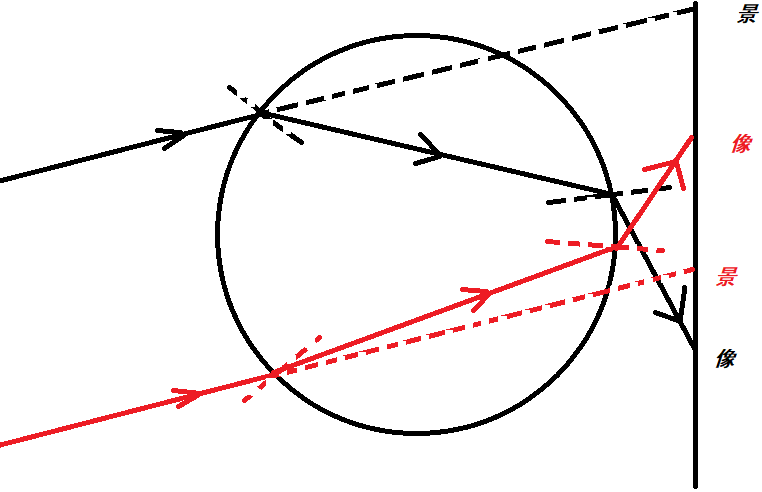
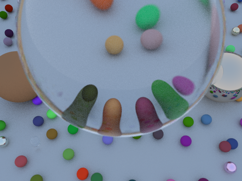
最后,我们实现的玻璃球球内图像是颠倒的,这属于正常现象,原因如下图所示。光线经过两次折射最终导致了图像的颠倒。
4、抗锯齿 为了减少光线追踪方法的噪声点和锯齿,我们需要做一些抗锯齿处理。方法就是在计算一个像素坐标的像素值时,发射很多条射线,射线的取值范围在一个像素之内,然后将所有光线获取的像素值累加起来,最后除以总的采样数。代码如下:
1
2
3
4
5
6
7
8
9
10
11
12
13
14
15
16
17
18
19
20
21
int samples = 100 ;for (int row = m_config.m_height - 1 ; row >= 0 ; --row){ for (int col = 0 ; col < m_config.m_width; ++col) { Vector4D color; for (int sps = 0 ; sps < samples; ++sps) { float u = static_cast <float >(col + drand48()) / static_cast <float >(m_config.m_width); float v = static_cast <float >(row + drand48()) / static_cast <float >(m_config.m_height); Ray ray = camera.getRay(u, v); color += tracing(ray, world, 0 ); } color /= static_cast <float >(samples); color.w = 1.0f ; color = Vector4D(sqrt (color.x), sqrt (color.y), sqrt (color.z), color.w); drawPixel(col, row, color); } }
这里还提到了gamma矫正,关于gamma矫正请看这里 )。我们对计算得到的像素做了一个简单的gamma矫正,gamma矫正系数取为$2.0$。不进行gamma矫正的话,渲染出来的图片明显偏暗。
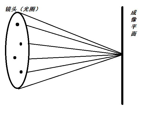
5、景深 关于现实生活中摄像机的景深原理,我不再详细说明。在光线追踪中实现景深并不复杂。实现的方法:首先是射线的出发点视点,我们的眼睛(或者相机)不再是一个点而是眼睛所在的周围圆盘上的随机点,因为实际的相机是有摄像镜头的,摄像镜头是一个大光圈(很大一个镜片),并不是针孔类的东东,所以,我们要模拟镜头,就要随机采针孔周围的光圈点。
此外还有一个焦距的问题,我们一开始假设成像平面在摄像机坐标系的$z=-1$上,为了实现摄像机的景深效果,现在我们要引入现实摄像机的焦距概念。简单的说焦距是焦点到面镜 的中心点之间的距离。因此我们提供了一个焦距的参数给用户调整,以确定所需的景深效果。通常情况下焦距$focusDist$等于$length(target-cameraPos)$。这个时候我们将成像平面挪到了摄像机坐标系的$z=-focusDist$上,相应地需要调整计算成像平面的$halfHeight$(在前面的基础上再乘上个$focusDist$)。
1 2 3 4 5 6 7 8 9 10 11 12 13 14 15 16 17 18 19 20 21 22 23 24 25 26 27 28 29 30 31 32 33 34 Camera::Camera(const Vector3D &cameraPos, const Vector3D &target, float vfov, float aspect, float aperture, float focus_dist) { m_pos = cameraPos; m_target = target; m_fovy = vfov; m_aspect = aspect; m_lensRadius = aperture * 0.5f ; m_focusDist = focus_dist; update(); } void Camera::update(){ const Vector3D worldUp (0.0f , 1.0f , 0.0f ) float theta = radians(m_fovy); float half_height = static_cast <float >(tan (theta * 0.5f )) * m_focusDist; float half_width = m_aspect * half_height; m_axisZ = m_pos - m_target; m_axisZ.normalize(); m_axisX = worldUp.crossProduct(m_axisZ); m_axisX.normalize(); m_axisY = m_axisZ.crossProduct(m_axisX); m_axisY.normalize(); m_lowerLeftCorner = m_pos - m_axisX * half_width - m_axisY * half_height - m_axisZ * m_focusDist; m_horizontal = m_axisX * 2.0f * half_width; m_vertical = m_axisY * 2.0f * half_height; }
6、递归光线追踪 最后,我们实现的光线追踪器$Tracer$如下,追踪器的核心实现主要在$tracing$函数和$render$函数。
1
2
3
4
5
6
7
8
9
10
11
12
13
14
15
16
17
18
19
20
21
22
23
24
25
26
27
28
29
30
31
32
33
34
35
36
37
38
39
40
41
42
43
44
45
46
47
48
49
50
51
52
53
54
55
56
57
58
59
60
61
62
63
64
65
66
67
68
69
70
71
72
73
74
75
76
77
78
79
80
81
82
83
84
85
86
87
88
89
90
91
92
93
94
95
96
97
98
99
100
101
102
103
104
105
106
107
108
109
110
111
112
113
114
115
116
117
118
119
120
121
122
123
124
125
126
127
128
129
130
131
132
133
134
135
136
137
138
139
140
141
142
143
144
145
146
147
148
149
150
151
152
153
154
155
156
157
158
159
160
161
162
163
164
165
166
167
168
class Hitable ;class Vector3D ;class Vector4D ;class Tracer { private : class Setting { public : int m_maxDepth; int m_width, m_height, m_channel; Setting():m_maxDepth(50 ), m_channel(4 ) {} }; Setting m_config; unsigned char *m_image; public : Tracer(); ~Tracer(); void initialize (int w, int h, int c = 4 ) unsigned char *render () int getWidth () const return m_config.m_width; } int getHeight () const return m_config.m_height; } int getChannel () const return m_config.m_channel; } int getRecursionDepth () const return m_config.m_maxDepth; } unsigned char *getImage () const return m_image; } void setRecursionDepth (int depth) void setCamera (const Vector3D &cameraPos, const Vector3D &target, const Vector3D &worldUp, float fovy, float aspect, float aperture, float focus_dist) private : Hitable *randomScene () ; Vector4D tracing (const Ray &r, Hitable *world, int depth) ; float hitSphere (const Vector3D ¢er, const float &radius, const Ray &ray) void drawPixel (unsigned int x, unsigned int y, const Vector4D &color) }; void Tracer::initialize(int w, int h, int c){ m_config.m_width = w; m_config.m_height = h; if (m_image != nullptr ) delete m_image; m_image = new unsigned char [m_config.m_width * m_config.m_height * m_config.m_channel]; } unsigned char *Tracer::render(){ Vector3D lower_left_corner (-2.0 , -1.0 , -1.0 ) ; Vector3D horizontal (4.0 , 0.0 , 0.0 ) ; Vector3D vertical (0.0 , 2.0 , 0.0 ) ; Vector3D origin (0.0 , 0.0 , 0.0 ) ; Hitable* world = randomScene(); Vector3D lookfrom (3 , 4 , 10 ) ; Vector3D lookat (0 , 0 , 0 ) ; float dist_to_focus = 10.0f ; float aperture = 0.0f ; Camera camera (lookfrom, lookat, 45 , static_cast <float >(m_config.m_width) / m_config.m_height, aperture, dist_to_focus) int samples = 100 ; for (int row = m_config.m_height - 1 ; row >= 0 ; --row) { for (int col = 0 ; col < m_config.m_width; ++col) { Vector4D color; for (int sps = 0 ; sps < samples; ++sps) { float u = static_cast <float >(col + drand48()) / static_cast <float >(m_config.m_width); float v = static_cast <float >(row + drand48()) / static_cast <float >(m_config.m_height); Ray ray = camera.getRay(u, v); color += tracing(ray, world, 0 ); } color /= static_cast <float >(samples); color.w = 1.0f ; color = Vector4D(sqrt (color.x), sqrt (color.y), sqrt (color.z), color.w); drawPixel(col, row, color); } } reinterpret_cast <HitableList*>(world)->clearHitable(); delete world; return m_image; } void Tracer::drawPixel(unsigned int x, unsigned int y, const Vector4D &color){ if (x < 0 || x >= m_config.m_width || y < 0 || y >= m_config.m_height) return ; unsigned int index = (y * m_config.m_width + x) * m_config.m_channel; m_image[index + 0 ] = static_cast <unsigned char >(255 * color.x); m_image[index + 1 ] = static_cast <unsigned char >(255 * color.y); m_image[index + 2 ] = static_cast <unsigned char >(255 * color.z); m_image[index + 3 ] = static_cast <unsigned char >(255 * color.w); } Hitable *Tracer::randomScene() { int n = 500 ; HitableList *list = new HitableList(); list ->addHitable(new Sphere(Vector3D(0 , -1000.0 , 0 ), 1000 , new Lambertian(Vector3D(0.5 , 0.5 , 0.5 )))); for (int a = -11 ; a < 11 ; ++a) { for (int b = -11 ; b < 11 ; ++b) { float choose_mat = drand48(); Vector3D center (a + 0.9 *drand48(), 0.2 , b + 0.9 *drand48()) ; if ((center - Vector3D(4 , 0.2 , 0 )).getLength() > 0.9 ) { if (choose_mat < 0.4f ) list ->addHitable(new Sphere(center, 0.2 , new Lambertian (Vector3D(drand48()*drand48(), drand48()*drand48(), drand48()*drand48())))); else if (choose_mat < 0.6f ) list ->addHitable(new Sphere(center, 0.2 , new Metal (Vector3D(0.5f *(1.0f + drand48()), 0.5f *(1.0f + drand48()), 0.5f *(1.0f + drand48())), 0.5f *drand48()))); else list ->addHitable(new Sphere(center, 0.2 , new Dielectric (1.5f ))); } } } list ->addHitable(new Sphere(Vector3D(0 , 1 , 0 ), 1.0 , new Dielectric(1.5f ))); list ->addHitable(new Sphere(Vector3D(-4 , 1 , 0 ), 1.0 , new Lambertian(Vector3D(0.4 , 0.2 , 0.1 )))); list ->addHitable(new Sphere(Vector3D(4 , 1 , 0 ), 1.0 , new Metal(Vector3D(0.7 , 0.6 , 0.5 ), 0.0f ))); return list ; } Vector4D Tracer::tracing(const Ray &r, Hitable *world, int depth) { HitRecord rec; if (world->hit(r, 0.001f , FLT_MAX, rec)) { Ray scattered; Vector3D attenuation; if (depth < m_config.m_maxDepth && rec.m_material->scatter(r, rec, attenuation, scattered)) return attenuation * tracing(scattered, world, depth + 1 ); else return Vector4D(0.0f , 0.0f , 0.0f , 1.0f ); } else { float t = 0.5f * (r.getDirection().y + 1.0f ); Vector4D ret = Vector3D(1.0f , 1.0f , 1.0f ) * (1.0f - t) + Vector3D(0.5f , 0.7f , 1.0f ) * t; ret.w = 1.0f ; return ret; } }
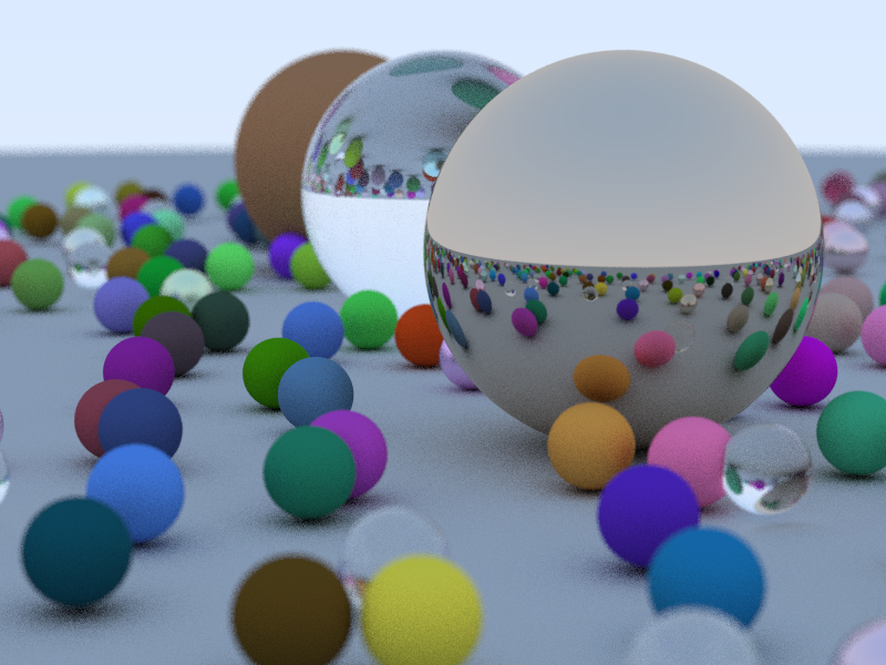
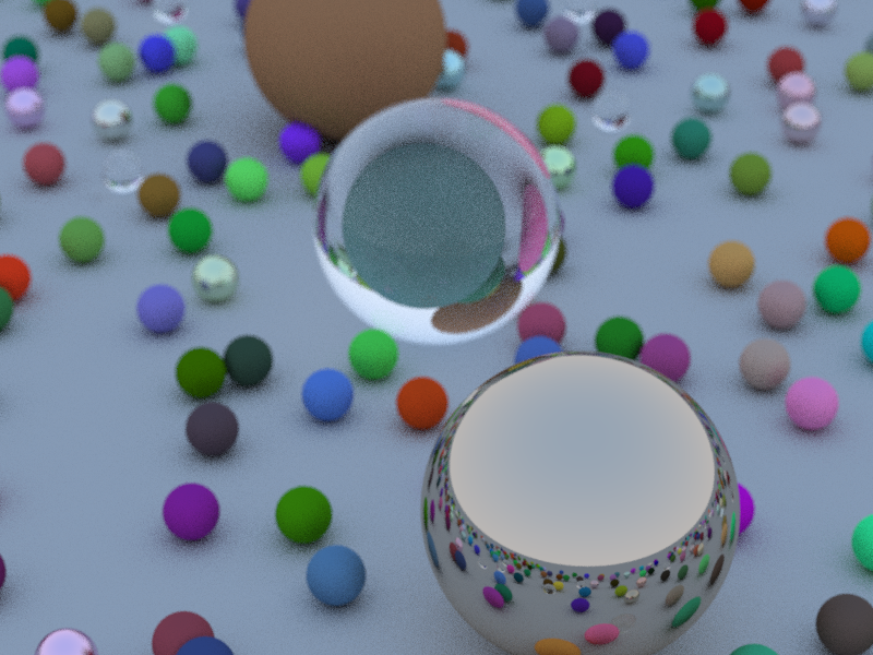
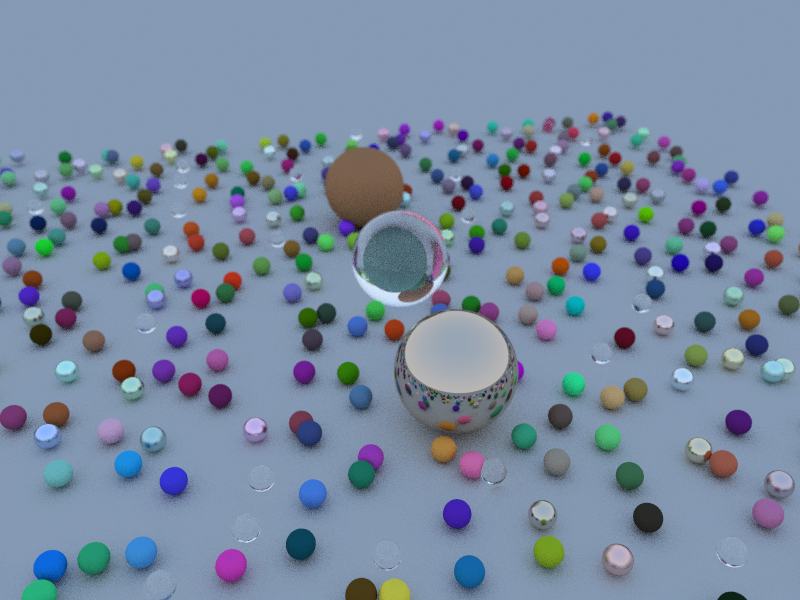
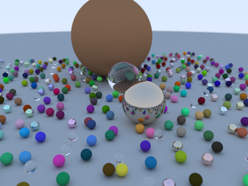
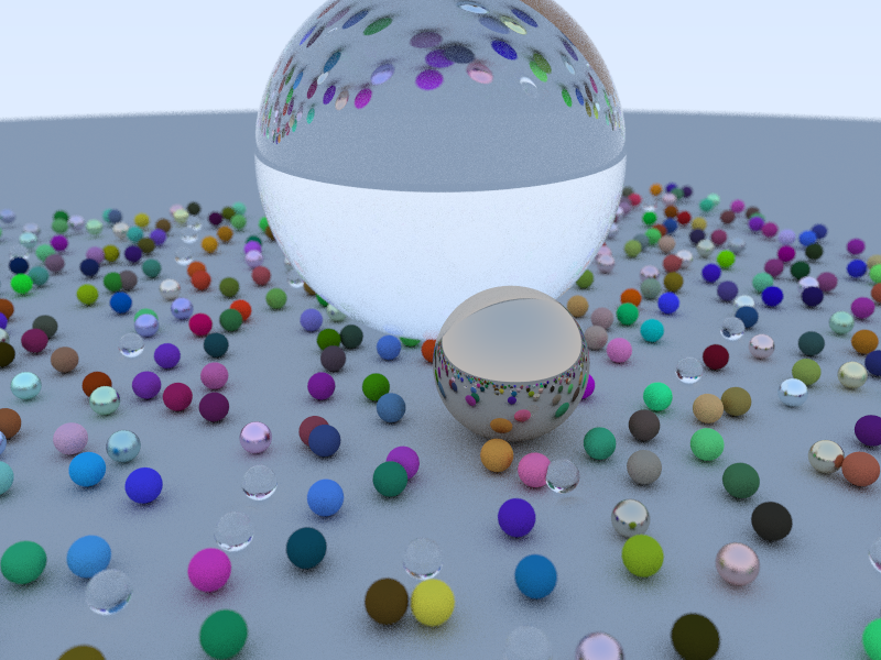
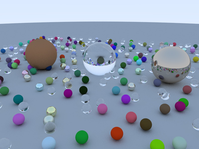
三、程序结果
参考资料 $[1]$ https://www.cnblogs.com/jerrycg/p/4941359.html
$[2]$ https://blog.csdn.net/baishuo8/article/details/81476422
$[3]$ https://blog.csdn.net/silangquan/article/details/8176855
$[4]$ Peter Shirley. Ray Tracing in One Weekend . Amazon Digital Services LLC, January 26, 2016.
$[5]$ https://learnopengl-cn.github.io/07%20PBR/01%20Theory/
$[6]$ https://www.cnblogs.com/lv-anchoret/p/10223222.html

,深入理解光线追踪的技术原理。主要参考资料为Peter Shirley的《Ray Tracing in One Weekend》。数学库沿用之前自己写的3D数学库,这方面的东西不再赘述。相关的完全代码在这里。
)
,深入理解光线追踪的技术原理。主要参考资料为Peter Shirley的《Ray Tracing in One Weekend》。数学库沿用之前自己写的3D数学库,这方面的东西不再赘述。相关的完全代码在这里。
)
,深入理解光线追踪的技术原理。主要参考资料为Peter Shirley的《Ray Tracing in One Weekend》。数学库沿用之前自己写的3D数学库,这方面的东西不再赘述。相关的完全代码在这里。
)