本篇承接上一篇《采样和重建(一)》,主要包含了分层抖动采样、Halton采样、(0,2)序列采样、最大最短距离采样和Sobol’采样方面的内容。
以下的内容大部分整理自pbrt第三版的第七章——SAMPLING AND RECONSTRUCTION。
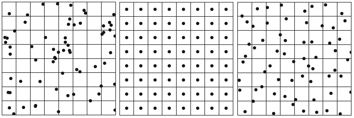
四、分层抖动采样 分层抖动采样就是在分层采样的基础上做随机抖动。分层采样(Stratified Sampling)本质上就是一维均匀采样的高维扩展,也就是高维的均匀采样方法。在此基础上,我们使得采样点做一些单个采样间隔内的随机偏移,从而达到即随机又总体上比较均匀分布的效果。以二维的采样为例,下图从左到右分别展示了随机采样、分层均匀采样、分层抖动采样的采样点分布情况。可以看到随机采样某些地方聚集、某些地方稀疏,分布得极其不理想;均匀采样均匀有规律地分布;在均匀采样的基础上做单个采样间隔内的随机抖动就得到了最右边的效果,相对于单纯的随机采样来说,采样点的分布均匀得多。
因此,分层抖动采样本质上就是前面提到的反走样技术中的非均匀采样方法,它尝试把走样的现象转换成噪声。对采样空间$[0,1)^n$的每一维做均匀的划分(即分层),每一维的一个划分相互组合得到采样空间中的均匀子空间(上图中就是一个小格子),这些子空间互不重叠,在每个这样的子空间做随机采样,从而完成整个分层抖动采样的过程,这就是分层抖动采样的大致思想。
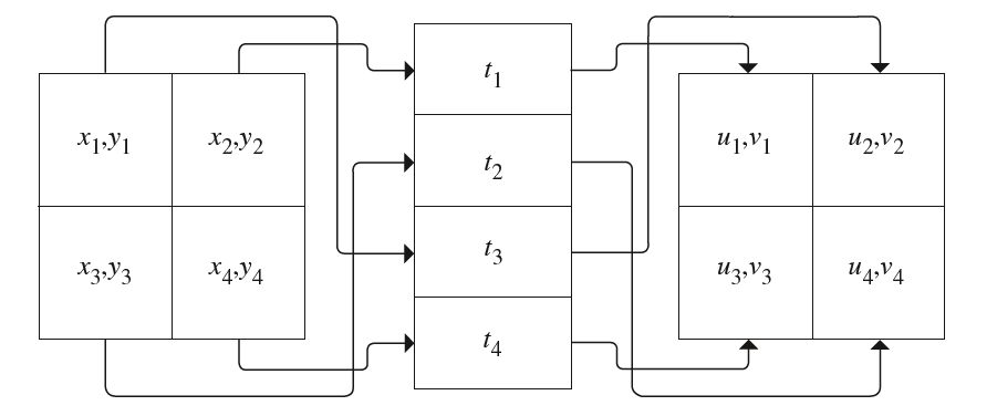
然后,理想的分层抖动采样很容易陷入维数灾难 (curse of dimensionality)的窘况。以五维采样空间为例(采样向量就是个五维向量),如果对每一维划分四层,则总共产生的子空间有$4^5=1024$,即我们要做$1024$次的采样。所以理想的分层抖动采样对于高维的采样空间不是很友好,因为维数越高,则划分的子空间数量呈指数增长。为此,人们想出了一种方法来解决这个问题,这种方法就是用一维和二维的分层抖动采样组合成高维的采样点。例如五维的采样空间,可以拆分成两维的采样、一维的采样和两维的采样。以摄像机需要的五个采样值$(x,y,t,u,v)$为例,如下图所示,我们分别在两维空间对$(x,y)$和$(u,v)$做分层抖动采样,在一维空间对$t$做分层抖动采样,分别得到四个低维的采样点,然后再将这些低维的采样点随机串起来得到一个五维的采样向量,例如$(x_2,y_2,t_1,u_1,v_1)$。注意这里的随机串联很重要。
随机串联的方法就是对每个低维的采样点做打乱顺序的洗牌过程,然后再逐个串起来即可。声明一个StratifiedSampler的采样器类如下:
1 2 3 4 5 6 7 8 9 10 11 12 13 14 15 16 17 class StratifiedSampler :public PixelSampler { public : StratifiedSampler(int xPixelSamples, int yPixelSamples, bool jitterSamples, int nSampledDimensions) : PixelSampler(xPixelSamples * yPixelSamples, nSampledDimensions), xPixelSamples(xPixelSamples), yPixelSamples(yPixelSamples), jitterSamples(jitterSamples) {} void StartPixel (const Point2i &) private : const int xPixelSamples, yPixelSamples; const bool jitterSamples; };
jitterSamples用于控制是否要做随机抖动,如果不抖动则就是分层的均匀采样。在StartPixel中一次性生成所有的采样点,StratifiedSample1D生成一个维度的随机抖动采样点,然后使用Shuffle对这些采样点进行随机打乱(这里的洗牌算法使用的是Knuth-Durstenfeld Shuffle 算法):
1
2
3
4
5
6
7
8
9
10
11
12
void StratifiedSampler::StartPixel(const Point2i &p) { for (size_t i = 0 ; i < samples1D.size(); ++i) { StratifiedSample1D(&samples1D[i][0 ], xPixelSamples * yPixelSamples, rng, jitterSamples); Shuffle(&samples1D[i][0 ], xPixelSamples * yPixelSamples, 1 , rng); } }
StratifiedSample1D的定义如下,二维同理:
1 2 3 4 5 6 7 8 void StratifiedSample1D (Float *samp, int nSamples, RNG &rng, bool jitter) Float invNSamples = (Float)1 / nSamples; for (int i = 0 ; i < nSamples; ++i) { Float delta = jitter ? rng.UniformFloat() : 0.5f ; samp[i] = std ::min((i + delta) * invNSamples, OneMinusEpsilon); } }
上面仅仅处理了一次只请求一个采样值的数据生成,接下来要处理一次性请求多个采样值的数据生成。例如某个积分器要求一次性获取$64$个二维采样向量,用这$64$个采样点对光源做重要性采样。这时我们要求这$64$个采样点在二维平面$[0,1)^2$上有良好的分布(分成$8\times 8=64$个子空间)。我们姑且称之为一个块,一个块要求的采样值数量不一,取决于使用场合。这个数量有时可能不太好对二维进行划分(例如$7$个)。一种方法就是强制使得数量为两个整数的相乘,例如令$7$变为$9=3\times 3$。
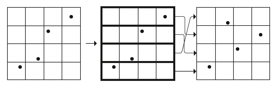
但pbrt提出了另一种采样方法解决这个问题,这个采样叫做拉丁超立方采样(Latin hypercube sampling,简称为LHS,亦被称为n-rook采样)。给定任意的待采样数量,它都能生成比较良好分布的采样点。以二维$[0,1)^2$为例,我们要在上面采样$4$个点,则将二维$[0,1)^2$空间划分成$4\times 4$个子空间,然后仅在那些对角线上的子空间中做随机采样,最后再在每一维度上对采样点随机打乱顺序。下图展示了这个过程:
因此,可以实现LatinHypercube方法如下:
1
2
3
4
5
6
7
8
9
10
11
12
13
14
15
16
void LatinHypercube (Float *samples, int nSamples, int nDim, RNG &rng) Float invNSamples = (Float)1 / nSamples; for (int i = 0 ; i < nSamples; ++i) for (int j = 0 ; j < nDim; ++j) { Float sj = (i + (rng.UniformFloat())) * invNSamples; samples[nDim * i + j] = std ::min(sj, OneMinusEpsilon); } for (int i = 0 ; i < nDim; ++i) { for (int j = 0 ; j < nSamples; ++j) { int other = j + rng.UniformUInt32(nSamples - j); std ::swap(samples[nDim * j + i], samples[nDim * other + i]); } } }
最后,分块获取的采样值生成中,一维的不需要借助于LatinHypercube(但需要按块生成采样,而不是像上面那样一次性生成一个维度的全部采样值),仅二维需要使用LatinHypercube方法。
1
2
3
4
5
6
7
8
9
10
11
12
13
14
15
16
17
18
19
void StratifiedSampler::StartPixel(const Point2i &p) { ... for (size_t i = 0 ; i < samples1DArraySizes.size(); ++i) for (int64_t j = 0 ; j < samplesPerPixel; ++j) { int count = samples1DArraySizes[i]; StratifiedSample1D(&sampleArray1D[i][j * count], count, rng, jitterSamples); Shuffle(&sampleArray1D[i][j * count], count, 1 , rng); } for (size_t i = 0 ; i < samples2DArraySizes.size(); ++i) for (int64_t j = 0 ; j < samplesPerPixel; ++j) { int count = samples2DArraySizes[i]; LatinHypercube(&sampleArray2D[i][j * count].x, count, 2 , rng); } ... }
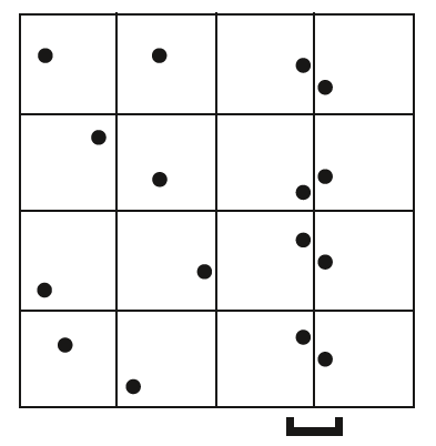
分层抖动采样方法产生的采样点分布比较均匀,不会出现过度的聚集现象,也不会有某些采样空间只拥有极少的采样点的情况。但它也有缺点,它仅考虑了整个采样空间的分布均匀情况,而忽略了单个维度上的采样点分布情况,因此有可能出现在某一维度上聚集的极端的情况,如下图所示:
五、Halton采样 Halton采样算法基于低差异性的点集合,在确保生成的点集整体上不会太过聚集的同时,又考虑采样点在单个维度上的分布情况。我们将借助Hammersley序列和Halton序列实现Halton采样器。
1、Hammersley序列和Halton序列 Hammersley序列和Halton序列是两个密切相关的低差异性点集。这两个序列的生成都依赖于逆根 (radical inverse)函数实现,它基于这样的一个事实:给定一个正整数$a$和基数$b$,$a$在基数$b$下的位序列记为$d_m(a)…d_2(a)d_1(a)$,$0\leq d_i(a)\leq b-1$则有:
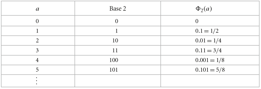
逆根函数$\Phi$根据给定的非负整数$a$和基数$b$,通过将$a$在基数$b$下的位序列以小数点为界镜像映射到$[0,1)$的浮点数:
一个最简单的低差异性序列就是van der Corput序列,它是由基数为$2$的逆根函数生成的一维序列$x_a=\Phi_2(a)$,下图展示了这样的一个序列。
在此基础上,我们定义$n$维的Halton序列,为了生成一个$n$维的采样向量,分别使用$n$个互素的素数$(p_1,…,p_n)$,每一维使用其对应一个素数$p_i$作为基数调用逆根函数$\Phi_{p_i}(a)$生成相应的采样值:
对于一个$n$维的低差异性序列,其差异性值满足$D_N^* (x_a)=O(\frac{(logN)^n}{N})$,逼近最优。设总b_的采样数量为$N$,$b_i$是第$i$个素数,则Hammersley点集被定义为:
给定基数base和非负整数a,可以很容易地用模板函数实现逆根函数如下所示:
1
2
3
4
5
6
7
8
9
10
11
12
13
14
template <int base>PBRT_NOINLINE static Float RadicalInverseSpecialized (uint64_t a) { const Float invBase = (Float)1 / (Float)base; uint64_t reversedDigits = 0 ; Float invBaseN = 1 ; while (a) { uint64_t next = a / base; uint64_t digit = a - next * base; reversedDigits = reversedDigits * base + digit; invBaseN *= invBase; a = next; } return std ::min(reversedDigits * invBaseN, OneMinusEpsilon); }
我们使用自然数中前$1000$个素数($2,3,5,7,…$)作为基数实例化模板函数,由于二进制的特殊性,这里对基数为$2$的情况做了优化,用ReverseBits64实现了专门用于基数为$2$的逆根函数计算:
1 2 3 4 5 6 7 8 9 10 11 12 13 14 15 16 17 18 19 Float RadicalInverse (int baseIndex, uint64_t a) { switch (baseIndex) { case 0 : #ifndef PBRT_HAVE_HEX_FP_CONSTANTS return ReverseBits64(a) * 5.4210108624275222e-20 ; #else return ReverseBits64(a) * 0x1 p-64 ; #endif case 1 : return RadicalInverseSpecialized<3 >(a); case 2 : return RadicalInverseSpecialized<5 >(a); case 3 : return RadicalInverseSpecialized<7 >(a); ...... } }
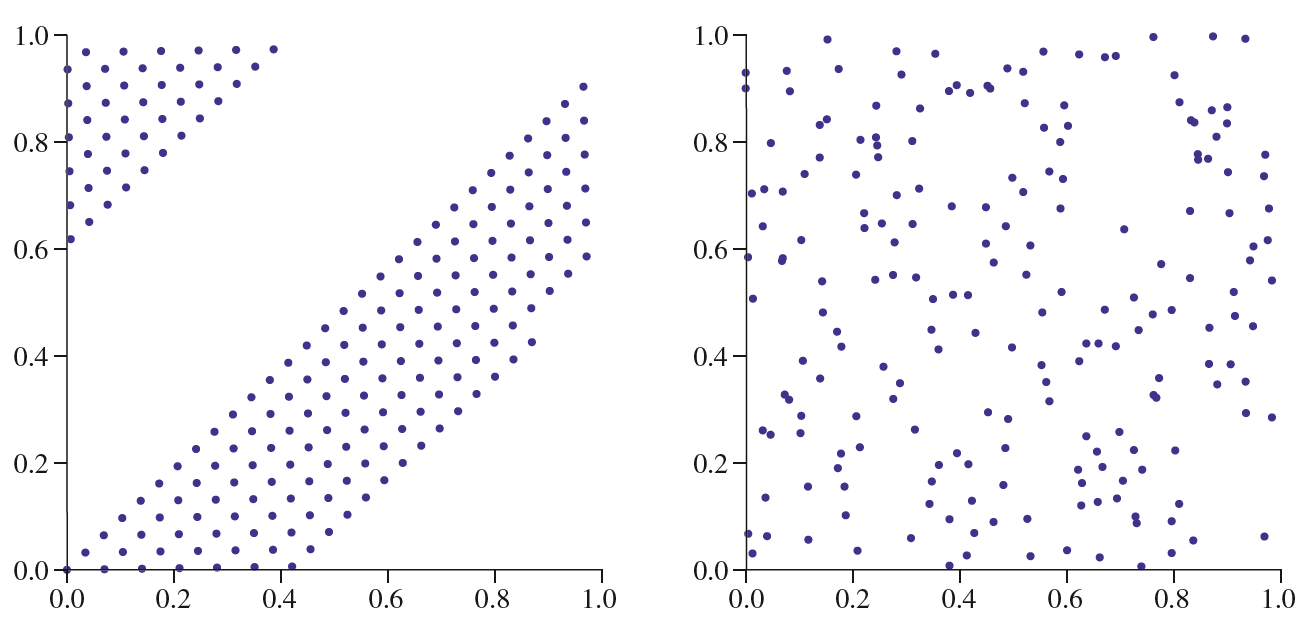
这样调用RadicalInverse就可以很方便地生成Hammersley序列和Halton序列。Hammersley序列和Halton序列的一个缺点就是随着基数$b$的增大,生成的采样点逐渐变得有规律起来,如下图左边所示。
为此,我们考虑在生成过程中对每一位进行一个随机扰动(上图右边是扰动的结果),记扰动算子为$p$,则添加了扰动算子的逆根函数返回值为:
每一位的数字位取值为$(0,1,…,b-1)$,扰动操作将$d_i(a)$映射到另一个位于$(0,1,…,b-1)$的随机一个。为了实现扰动,我们预先生成一个扰动表perms,perms的前两个用于基数为$2$的扰动映射,紧接着的三个用于基数为$3$的扰动映射,依次类推。
1
2
3
4
5
6
7
8
9
10
11
12
13
14
15
std ::vector <uint16_t > ComputeRadicalInversePermutations(RNG &rng) { std ::vector <uint16_t > perms; int permArraySize = 0 ; for (int i = 0 ; i < PrimeTableSize; ++i) permArraySize += Primes[i]; perms.resize(permArraySize); uint16_t *p = &perms[0 ]; for (int i = 0 ; i < PrimeTableSize; ++i) { for (int j = 0 ; j < Primes[i]; ++j) p[j] = j; Shuffle(p, Primes[i], 1 , rng); p += Primes[i]; } return perms; }
因此,有了随机扰动表,则对于每一位数字$d_i$,$perms[start+d_i]$(对应下面代码中的perm[digit])就是该位扰动映射的结果。最后的invBase * perm[0] / (1 - invBase))考虑了最高位前面的零。
1
2
3
4
5
6
7
8
9
10
11
12
13
14
15
16
17
18
19
20
template <int base>PBRT_NOINLINE static Float ScrambledRadicalInverseSpecialized(const uint16_t *perm, uint64_t a) { const Float invBase = (Float)1 / (Float)base; uint64_t reversedDigits = 0 ; Float invBaseN = 1 ; while (a) { uint64_t next = a / base; uint64_t digit = a - next * base; CHECK_LT(perm[digit], base); reversedDigits = reversedDigits * base + perm[digit]; invBaseN *= invBase; a = next; } DCHECK_LT(invBaseN * (reversedDigits + invBase * perm[0 ] / (1 - invBase)), 1.00001 ); return std ::min( invBaseN * (reversedDigits + invBase * perm[0 ] / (1 - invBase)), OneMinusEpsilon); }
2、Halton采样器的实现 Halton采样器基于Halton序列实现,相比于分层抖动采样,它的采样操作没有使用伪随机数。因此Halton采样的方法有可能出现走样现象而不是噪声。Halton序列的采样是一种全局采样器,设总共的像素数为$m$,每个像素的采样数量为$k$,每个采样向量维数为$d$,则它利用Halton序列生成$m\times k$个采样。每个采样都有一个全局索引$0,1,…,m\times k-1$,第$j$个采样向量的第$i$个维度使用扰动的Halton序列生成采样值$p(\Phi_{b_i}(j))$,注意根逆函数的输入是采样向量编号$j$和第$i$个素数。大致的实现思路就是这样。
因此我们要构建像素坐标$(x,y)$和该像素获取的采样向量的全局索引$s$的对应关系。对于每一个采样向量,该向量的前两维用于构建这种对应关系。以第一个采样向量为例,其全局索引$s=0$,注意到前两维的采样值分别由$\Phi_2(s=0)$和$\Phi_3(s=0)$生成(使用的基数分别为$2$和$3$)。假设像素的宽$w=2^j$、高$h=3^k$,则总共的像素数量为$2^j\times 3^k$,想办法把$x$和$\Phi_2(s=0)$关联起来,$y$同理。设$\Phi_2(s=0)=0.d_1(0)d_2(0)…d_j(0)…d_m(0)$,则将$\Phi_2(0)$和$2^j$相乘得$d_1(0)d_2(0)…d_j(0).d_{j+1}(0)…d_m(0)$,取这里的整数部分$d_1(0)d_2(0)…d_j(0)$与像素坐标的$x$对应起来,因为$d_1(0)d_2(0)…d_j(0)$取值在$[0,2^j-1]$,刚好对应图像的宽度(即横向的像素数量)。
总共生成$2^j\times 3^k\times spp$,$spp$是每个像素的采样数量,这些采样数量每隔$2^j\times 3^k$作为一组全部像素的单个采样点集合。例如某个像素的初始的采样点索引为$2$,则下一个应该是$2^j\times 3^k+2$,再下一个应该是$2^j\times 3^k+3$,依次类推下去。创建HaltonSampler类如下:
1
2
3
4
5
6
7
8
9
10
11
12
13
14
15
16
17
18
19
20
21
22
23
24
25
26
27
28
29
30
class HaltonSampler :public GlobalSampler { public : HaltonSampler(int nsamp, const Bounds2i &sampleBounds, bool sampleAtCenter = false ); int64_t GetIndexForSample(int64_t sampleNum) const ; Float SampleDimension (int64_t index, int dimension) const ; std ::unique_ptr <Sampler> Clone(int seed); private : static std ::vector <uint16_t > radicalInversePermutations; Point2i baseScales, baseExponents; int sampleStride; int multInverse[2 ]; mutable Point2i pixelForOffset = Point2i(std ::numeric_limits<int >::max(), std ::numeric_limits<int >::max()); mutable int64_t offsetForCurrentPixel; bool sampleAtPixelCenter; const uint16_t *PermutationForDimension (int dim) const if (dim >= PrimeTableSize) LOG(FATAL) << StringPrintf("HaltonSampler can only sample %d " "dimensions." , PrimeTableSize); return &radicalInversePermutations[PrimeSums[dim]]; } };
radicalInversePermutations是前面提到的扰动映射表,baseScales存储$(2^i,3^k)$,baseExponents存储$(i,k)$,sampleStride存储$2^j\times 3^k$。offsetForCurrentPixel存储当前像素的第一个采样点的全局索引值,后续该像素的第i个采样点的索引就可以通过offsetForCurrentPixel+sampleStride*i得到。采样点的全局索引用于输入根逆函数获取采样值。如果图像的宽度不是$2$的幂次方,我们就寻找第一个大于宽度的$2$的幂次方值,作为$2^i$,高度同理。SampleDimension获取采样点的全局索引,返回采样向量对应维度dim的采样值:
1
2
3
4
5
6
7
8
9
10
Float HaltonSampler::SampleDimension(int64_t index, int dim) const { if (sampleAtPixelCenter && (dim == 0 || dim == 1 )) return 0.5f ; if (dim == 0 ) return RadicalInverse(dim, index >> baseExponents[0 ]); else if (dim == 1 ) return RadicalInverse(dim, index / baseScales[1 ]); else return ScrambledRadicalInverse(dim, index, PermutationForDimension(dim)); }
六、(0,2)序列采样 (0,2)序列采样也是一种特殊的低差异性序列,与分层抖动采样相比,它生成的采样分布情况更加优良。以基数$2$对二维空间$[0,1)^2$进行分割(其实就是二分),取两个非负整数$l_1$和$l_2$作为分割深度,则分割的区间集合为:
其中$a_i=0,1,2,4,…,2^{l_i-1}$。(0,2)序列生成的$2^{l_1+l_2}$个采样中,上述的区间都将包含一个采样点,分布情况非常优秀。每生成$2^{l_1+l_2}$个 采样点都符合上述情况,因此以$2^{l_1+l_2}$个采样点作为一个批次,逐个批次为不同的像素生成采样点。(0,2)序列本质上是Sobol序列的前两维,它也用到了前面的根逆函数。但是考虑到根逆函数为不同基数(大于$2$的基数)的计算的计算量有点过于庞大,考虑将大于$2$的基数的逆根计算转换成基数为$2$的逆根计算。一种高效的方法就是使用生成矩阵(generator matrices) 将其他不同基数的逆根计算转换到同一个基数下的逆根计算。
设基数为$b$,非负整数$a$的位数为$n$,第$i$位为$d_i(a)$,我们有一个$n\times n$的生成矩阵$C$,则可以生成$x_a\in [0,1)$的采样点如下:
若生成矩阵$C$为单位矩阵,则上述的公式等价于前面我们提到的常规的根逆计算。在这里,我们仅将实现基数$b=2$和$n=32$的生成矩阵。基数为$2$时,生成矩阵的元素取值为$0$或者$1$,因此生成矩阵的一列可以用一个$32$为的非负整数表示。根据矩阵向量乘法定义,则上面的矩阵向量相乘$C[d_i(a)]^T$可写成:
$d_i$也是取值为$0$或者$1$,因此上面的矩阵向量相乘等价于将$d_i$为$1$的对应的矩阵的那一列全部加起来,因为我们用一个$32$位整数表示矩阵的一列,所以这些列的相加等价于这些整数的异或。由此可以非常高效实现矩阵向量相乘的过程:
1
2
3
4
5
6
inline uint32_t MultiplyGenerator (const uint32_t *C, uint32_t a) uint32_t v = 0 ; for (int i = 0 ; a != 0 ; ++i, a >>= 1 ) if (a & 1 ) v ^= C[i]; return v; }
矩阵向量相乘MultiplyGenerator的结果$v$再与$[b^{-1} b^{-2} … b^n]$相乘等价于将$v$做二进制位的镜像翻转再除以$2^{32}$,这样就得到了我们所需的采样值$x_a$。为了进一步减少位翻转的开销,pbrt里在传入MultiplyGenerator之前先将生成矩阵的每一列做了位翻转,因为生成矩阵是预计算好的,这样后面就不用再翻转了。整个过程只涉及到一些移位运算和异或操作,非常高效。
同样为了加入随机性,我们给MultiplyGenerator的返回值做一个位扰动。扰动算法的设计需要非常小心,以防丢失了(0,2)序列的低差异性属性。具体的扰动算法这里不说了,扰动的实现可以直接用一个预先生成好的扰动序列scramble(用$32$位整数表示)与返回值v进行异或,如下所示,Float(0x1p-32)是$2^{-32}$:
1
2
3
4
5
inline Float SampleGeneratorMatrix (const uint32_t *C, uint32_t a, uint32_t scramble = 0 ) return std ::min((MultiplyGenerator(C, a) ^ scramble) * Float(0x1 p-32 ), OneMinusEpsilon); }
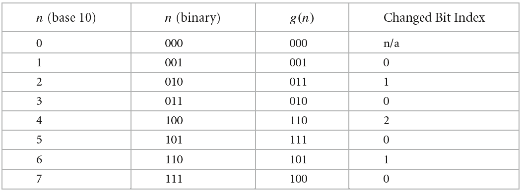
上面给出了一种高效的采样值计算过程。但pbrt指出,我们可以实现更高效的采样值生成过程。更高效的实现是从生成采样值的过程中以格雷码(gray code)的顺序执行入手。对于$n$位的$a$,$a$的取值范围为$0$到$2^n-1$,格雷码以一种特殊的顺序枚举$0$到$2^n-1$之间的数字,这种特殊的顺序表现在两个相邻的格雷码之间仅有一个二进制位不同 ,如下图的$g(n)$所示:
由此,假设对于$a$,我们已经计算得到了$v=C[d_i(a)]^T$,那么对于与$a$只有一个二进制位不同的$a’$的$v’=C[d_I(a’)]^T$的计算,我们只需在$v$的基础上加上或减去(通过异或实现)该不同二进制位对应的矩阵的那一列。所以关键是找到不同的那一个二进制位,这个比较技巧性,就不赘述了。下面是GrayCodeSample方法,与SampleGeneratorMatrix只生成给定的a对应的采样值不同,它输入$n$,生成$0$到$2^n-1$之间所有整数值对应的采样值,结果保存到$p$数组中,通过以格雷码的顺序枚举加速整个生成过程。
1
2
3
4
5
6
7
8
inline void GrayCodeSample (const uint32_t *C, uint32_t n, uint32_t scramble, Float *p) uint32_t v = scramble; for (uint32_t i = 0 ; i < n; ++i) { p[i] = std ::min(v * Float(0x1 p-32 ) , OneMinusEpsilon); v ^= C[CountTrailingZeros(i + 1 )]; } }
上面讨论的都是一维的采样值生成过程,二维就是多加了一个生成矩阵C1,差别不大。
1
2
3
4
5
6
7
8
9
10
inline void GrayCodeSample (const uint32_t *C0, const uint32_t *C1, uint32_t n, const Point2i &scramble, Point2f *p) uint32_t v[2 ] = {(uint32_t )scramble.x, (uint32_t )scramble.y}; for (uint32_t i = 0 ; i < n; ++i) { p[i].x = std ::min(v[0 ] * Float(0x1 p-32 ), OneMinusEpsilon); p[i].y = std ::min(v[1 ] * Float(0x1 p-32 ), OneMinusEpsilon); v[0 ] ^= C0[CountTrailingZeros(i + 1 )]; v[1 ] ^= C1[CountTrailingZeros(i + 1 )]; } }
紧接着用上述的相关函数创建ZeroTwoSequenceSampler的(0,2)序列采样器,这个采样器对于摄像机的五个采样值(即$(x,y,t,u,v)$)以及其他二维的采样值使用扰动的(0,2)序列生成,剩下的一维采样值使用扰动的van der Corput序列生成(就是基数为$2$的根逆函数生成的序列)。
1
2
3
4
5
6
7
8
class ZeroTwoSequenceSampler :public PixelSampler { public : ZeroTwoSequenceSampler(int64_t samplesPerPixel, int nSampledDimensions = 4 ); void StartPixel (const Point2i &) std ::unique_ptr <Sampler> Clone(int seed); int RoundCount (int count) const return RoundUpPow2(count); } };
(0,2)序列采样器需要确保每个像素的采样数量为$2$的幂次方,如果不是就使得采样数量为第一个大于当前采样数量的$2$幂次方,即下面的RoundUpPow2函数,因为这样能够使得(0,2)序列生成得采样点分布更加优良:
1 2 3 4 5 6 7 8 9 ZeroTwoSequenceSampler::ZeroTwoSequenceSampler(int64_t samplesPerPixel, int nSampledDimensions) : PixelSampler(RoundUpPow2(samplesPerPixel), nSampledDimensions) { if (!IsPowerOf2(samplesPerPixel)) Warning( "Pixel samples being rounded up to power of 2 " "(from %" PRId64 " to %" PRId64 ")." , samplesPerPixel, RoundUpPow2(samplesPerPixel)); }
对于一维的采样点,将使用前面的GrayCodeSample生成van der Corput序列,van der Corput序列本身就是由基数为$2$的根逆函数生成,因此生成矩阵就是一个单位矩阵。下面的CVanDerCorput数组保存了生成矩阵的每一列,它的每一列都预先翻转了。
1
2
3
4
5
6
7
8
9
10
11
12
13
14
15
16
17
18
19
20
21
inline void VanDerCorput (int nSamplesPerPixelSample, int nPixelSamples, Float *samples, RNG &rng) uint32_t scramble = rng.UniformUInt32(); const uint32_t CVanDerCorput[32 ] = { 0b10000000000000000000000000000000 , 0b1000000000000000000000000000000 , 0b100000000000000000000000000000 , 0b10000000000000000000000000000 , ... }; int totalSamples = nSamplesPerPixelSample * nPixelSamples; GrayCodeSample(CVanDerCorput, totalSamples, scramble, samples); for (int i = 0 ; i < nPixelSamples; ++i) Shuffle(samples + i * nSamplesPerPixelSample, nSamplesPerPixelSample, 1 , rng); Shuffle(samples, nPixelSamples, nSamplesPerPixelSample, rng); }
为了防止生成的采样点之间存在某种意想不到的关联,生成的采样序列需要被Shuffle进行一个随机洗牌过程。对于二维的采样值,这里将使用Sobol序列的生成矩阵调用GrayCodeSample。如下所示:
1
2
3
4
5
6
7
8
9
10
11
12
13
14
15
16
17
18
19
20
21
22
23
24
25
inline void Sobol2D (int nSamplesPerPixelSample, int nPixelSamples, Point2f *samples, RNG &rng) Point2i scramble; scramble[0 ] = rng.UniformUInt32(); scramble[1 ] = rng.UniformUInt32(); const uint32_t CSobol[2 ][32 ] = { {0x80000000 , 0x40000000 , 0x20000000 , 0x10000000 , 0x8000000 , 0x4000000 , 0x2000000 , 0x1000000 , 0x800000 , 0x400000 , 0x200000 , 0x100000 , 0x80000 , 0x40000 , 0x20000 , 0x10000 , 0x8000 , 0x4000 , 0x2000 , 0x1000 , 0x800 , 0x400 , 0x200 , 0x100 , 0x80 , 0x40 , 0x20 , 0x10 , 0x8 , 0x4 , 0x2 , 0x1 }, {0x80000000 , 0xc0000000 , 0xa0000000 , 0xf0000000 , 0x88000000 , 0xcc000000 , 0xaa000000 , 0xff000000 , 0x80800000 , 0xc0c00000 , 0xa0a00000 , 0xf0f00000 , 0x88880000 , 0xcccc0000 , 0xaaaa0000 , 0xffff0000 , 0x80008000 , 0xc000c000 , 0xa000a000 , 0xf000f000 , 0x88008800 , 0xcc00cc00 , 0xaa00aa00 , 0xff00ff00 , 0x80808080 , 0xc0c0c0c0 , 0xa0a0a0a0 , 0xf0f0f0f0 , 0x88888888 , 0xcccccccc , 0xaaaaaaaa , 0xffffffff }}; GrayCodeSample(CSobol[0 ], CSobol[1 ], nSamplesPerPixelSample * nPixelSamples, scramble, samples); for (int i = 0 ; i < nPixelSamples; ++i) Shuffle(samples + i * nSamplesPerPixelSample, nSamplesPerPixelSample, 1 , rng); Shuffle(samples, nPixelSamples, nSamplesPerPixelSample, rng); }
最后,在StartPixel中使用这里两个函数生成所需的采样点。
1
2
3
4
5
6
7
8
9
10
11
12
13
14
15
16
17
void ZeroTwoSequenceSampler::StartPixel(const Point2i &p) { ProfilePhase _(Prof::StartPixel); for (size_t i = 0 ; i < samples1D.size(); ++i) VanDerCorput(1 , samplesPerPixel, &samples1D[i][0 ], rng); for (size_t i = 0 ; i < samples2D.size(); ++i) Sobol2D(1 , samplesPerPixel, &samples2D[i][0 ], rng); for (size_t i = 0 ; i < samples1DArraySizes.size(); ++i) VanDerCorput(samples1DArraySizes[i], samplesPerPixel, &sampleArray1D[i][0 ], rng); for (size_t i = 0 ; i < samples2DArraySizes.size(); ++i) Sobol2D(samples2DArraySizes[i], samplesPerPixel, &sampleArray2D[i][0 ], rng); PixelSampler::StartPixel(p); }
七、最大最短距离采样 (0,2)序列有时生成的采样点也会过于聚集,一种可行的解决方案就是使用一对不同的生成矩阵,使得既可以生成良好分布的(0,2)序列,又可以最大化采样点之间的最短距离。下面将实现一个最大最短距离采样器MaxMinDistSampler:
1
2
3
4
5
6
7
8
9
class MaxMinDistSampler :public PixelSampler { public : ... private : const uint32_t *CPixel; };
这里实现的最大最短距离采样与(0,2)序列采样区别不是很大,主要的区别在于使用了一个特殊的生成器矩阵。这些生成器矩阵的获取比较复杂,直接从相关的paper中拿出来保存到CMaxMinDist中。下面的变量保存了17个生成矩阵,分别对应着像素采样数量为$2^0,2^1,2^2,…,2^{15},2^{16}$,例如单个像素的采样数量为$2^5$,则获取CMaxMinDist[5]作为特殊的生成矩阵保存到CPixel中。
1 extern uint32_t CMaxMinDist[17 ][32 ];
对于非$2$幂次数量的情况,则用Log2Int方法计算其矩阵的下标,并用RoundUpPow2变成大于当前数量的第一个$2$幂次方。(注意,采样数量上限为$2^{16}$)。
1 2 3 4 5 6 7 8 9 10 11 12 13 MaxMinDistSampler(int64_t samplesPerPixel, int nSampledDimensions) : PixelSampler([](int64_t spp) { if (!IsPowerOf2(spp)) { spp = RoundUpPow2(spp); Warning("Non power-of-two sample count rounded up to %" PRId64 " for MaxMinDistSampler." , spp); } return spp; }(samplesPerPixel), nSampledDimensions) { int Cindex = Log2Int(samplesPerPixel); CPixel = CMaxMinDist[Cindex]; }
它生成采样点的过程是这样的。对于第一个维度的二维的采样值,用Point2f(i * invSPP, SampleGeneratorMatrix(CPixel, i))生成,剩余的照搬前面的(0,2)序列采样。(应该是为了像素内的偏移$(x,y)$量身定做的,因为第一个维度一般用于像素内偏移的采样)
1
2
3
4
5
6
7
8
9
10
11
12
13
14
15
16
17
18
19
20
21
22
23
void MaxMinDistSampler::StartPixel(const Point2i &p) { Float invSPP = (Float)1 / samplesPerPixel; for (int i = 0 ; i < samplesPerPixel; ++i) samples2D[0 ][i] = Point2f(i * invSPP, SampleGeneratorMatrix(CPixel, i)); Shuffle(&samples2D[0 ][0 ], samplesPerPixel, 1 , rng); for (size_t i = 0 ; i < samples1D.size(); ++i) VanDerCorput(1 , samplesPerPixel, &samples1D[i][0 ], rng); for (size_t i = 1 ; i < samples2D.size(); ++i) Sobol2D(1 , samplesPerPixel, &samples2D[i][0 ], rng); for (size_t i = 0 ; i < samples1DArraySizes.size(); ++i) { int count = samples1DArraySizes[i]; VanDerCorput(count, samplesPerPixel, &sampleArray1D[i][0 ], rng); } for (size_t i = 0 ; i < samples2DArraySizes.size(); ++i) { int count = samples2DArraySizes[i]; Sobol2D(count, samplesPerPixel, &sampleArray2D[i][0 ], rng); } PixelSampler::StartPixel(p); }
八、Sobol’ 采样 (0,2)序列采样在Halton采样的基础上改进,仅使用基数为$2$的根逆函数,而且使用不同的生成矩阵,但它仅考虑一维和两维的情况。由此,考虑全部维度使用不同的生成矩阵,就是Sobol序列的采样方法。Sobol序列也只考虑基数为$2$的根逆函数,采样向量的每个维度都有格子不同的生成矩阵$C$。生成矩阵的获取由特殊的算法得到,这里 给出了Sobol序列的预计算好的生成矩阵,可以直接拿来用。下面实现了Sobol采样,它的关键点就是生成矩阵的SobolMatrices32,其他和前面的Halton采样一样:
1
2
3
4
5
6
inline float SobolSampleFloat (int64_t a, int dimension, uint32_t scramble) uint32_t v = scramble; for (int i = dimension * SobolMatrixSize; a != 0 ; a >>= 1 , i++) if (a & 1 ) v ^= SobolMatrices32[i]; return std ::min(v * 0x1 p-32f , FloatOneMinusEpsilon); }
Sobol’采样在各个维度上使用不同的生成矩阵,因此具备优良的分布。但是它的缺点就是在收敛之前容易出现网格结构状的失真现象。下面实现一个Sobol’采样器,注意它是一个全局采样器:
1
2
3
4
5
6
7
8
9
10
11
12
13
14
15
16
17
18
19
20
21
22
23
class SobolSampler :public GlobalSampler { public : std ::unique_ptr <Sampler> Clone(int seed); SobolSampler(int64_t samplesPerPixel, const Bounds2i &sampleBounds) : GlobalSampler(RoundUpPow2(samplesPerPixel)), sampleBounds(sampleBounds) { if (!IsPowerOf2(samplesPerPixel)) Warning("Non power-of-two sample count rounded up to %" PRId64 " for SobolSampler." , this ->samplesPerPixel); resolution = RoundUpPow2( std ::max(sampleBounds.Diagonal().x, sampleBounds.Diagonal().y)); log2Resolution = Log2Int(resolution); } int64_t GetIndexForSample(int64_t sampleNum) const ; Float SampleDimension (int64_t index, int dimension) const ; private : const Bounds2i sampleBounds; int resolution, log2Resolution; };
这里的一个实现难点依旧跟Halton采样一样,就是如何将像素坐标与采样向量的全局索引的映射建立起来。依旧用采样向量的前两维$[0,1)^2$与像素坐标联系起来。设图像的宽高$(w,h)=(2^i,2^j)$,如果不是$2$的幂次方则做一个RoundUpPow2,令log2Resolution=max(i,j),sampleBounds是像素的坐标范围。理论上,将前两维$[0,1)^2$乘上$2^{log2Resolution}$就可以得到采样向量与像素坐标的映射关系。但通常情况下我们是已知像素坐标要获取采样向量,因此要实现的是逆映射,具体细节这里不展开。
因为前两维用于像素坐标与采样向量的映射,因此获取时要做一些额外的处理(返回相对于当前像素的偏移量)。
1
2
3
4
5
6
7
8
9
Float SobolSampler::SampleDimension(int64_t index, int dim) const { Float s = SobolSample(index, dim); if (dim == 0 || dim == 1 ) { s = s * resolution + sampleBounds.pMin[dim]; s = Clamp(s - currentPixel[dim], (Float)0 , OneMinusEpsilon); } return s; }
Reference $[1]$ M, Jakob W, Humphreys G. Physically based rendering: From theory to implementation[M]. Morgan Kaufmann, 2016.
 | YangWC's Blog&pics=https://cdn.jsdelivr.net/gh/ZeusYang/CDN-for-yangwc.com@1.1.42/blog/TinySoftRenderer/renderer2.jpg&summary=本篇承接上一篇《采样和重建(一)》,主要包含了分层抖动采样、Halton采样、(0,2)序列采样、最大最短距离采样和Sobol’采样方面的内容。)
 | YangWC's Blog&pics=https://cdn.jsdelivr.net/gh/ZeusYang/CDN-for-yangwc.com@1.1.42/blog/TinySoftRenderer/renderer2.jpg&summary=本篇承接上一篇《采样和重建(一)》,主要包含了分层抖动采样、Halton采样、(0,2)序列采样、最大最短距离采样和Sobol’采样方面的内容。)
 | YangWC's Blog&pics=https://cdn.jsdelivr.net/gh/ZeusYang/CDN-for-yangwc.com@1.1.42/blog/TinySoftRenderer/renderer2.jpg&summary=本篇承接上一篇《采样和重建(一)》,主要包含了分层抖动采样、Halton采样、(0,2)序列采样、最大最短距离采样和Sobol’采样方面的内容。)