流体模拟Fluid Simulation：基于SPH的拉格朗日流体模拟

本文主要是关于拉格朗日粒子的流体模拟经典算法——SPH。

• 光滑粒子动力学
• SPH流体模拟算法
• PCISPH流体模拟算法
• 参考资料

基于SPH的拉格朗日流体模拟

  SPH，全称为Smoothed Particle Hydrodynamics，最初提出于天体物理学领域，然后被广泛的应用到计算流体力学领域，成为基于拉格朗日粒子模拟方法的典型代表。实际上，目前除了流体，还有刚体、软体等的物理模拟也有不少采用了SPH的方法。SPH是一种基于光滑粒子核的物理模型，它将模拟的对象离散成一个个粒子，然后以光滑核将粒子之间联系起来，显然这是一种基于拉格朗日视角的模拟方法，相对于欧拉视角的模拟方法，它比较简单、速度较快。

图1 基于粒子的流体模拟

一、光滑粒子动力学

  SPH的核心在于它的光滑核函数，首先我们来看看光滑核函数的推导。对于一个标量函数$f$，给定一个积分区域，有：

$$f(x)=\int f(y)\delta (x-y)dy \tag {1}$$

  且$\delta$是一个狄拉克函数，故上式$(1)$成立：

$$\delta (x-y)= \{ \begin{matrix} \infty\ \ ,x=y\\ 0\ \ \ \ ,x\neq y \end{matrix} \tag {2}$$

  将公式$(1)$中的狄拉克函数替换成一个光滑的核函数$\omega$：

$$f(x)\approx \int f(y)\omega (||x-y||/h)dy \tag {3}$$

  其中$h$是光滑核的半径长度，光滑核函数$\omega$具有以下的性质：

• 当$||w-y||/h >1$时，$w=0$，即超出核半径之外的定义域，函数值均取零。
• $lim_{h\to 0}w(||x-y||/h)=\delta (x-y)$，即当核半径$h$趋于零时，核函数收敛到公式$(2)$的狄拉克函数。
• 归一化条件，$\int w(||x-y||/h)dy=1$。
• 函数$\omega$是光滑连续的，因而是可微的。

  通过公式$(3)$，我们可以根据周围邻域的函数值近似获取给定的点的函数值，这些函数值可以是密度、压强等流体的属性值。公式$(3)$给出的是一个积分形式，在二维空间中的积分变量是面积，在三维空间中的积分变量是体积，我们采用黎曼和来离散地计算公式$(3)$：

$$\begin{align} f(x)\approx &\int f(y)\omega (||x-y||/h)dy\\ \approx &\Sigma_{i=1}^N f_i w(||x-x_i||/h_i)V_i\\ \approx &\Sigma_{i=1}^N \frac{m_i}{\rho_i}f_i w(||x-x_i||/h_i) \end{align} \tag {4}$$

  其中$V_i$是我们取的体积微元，又因$\rho=\frac mv$，所以最终可以写成如上所示的计算公式。$f_i$是第$i$个邻域粒子的函数取值。公式$(4)$并不需要我们遍历在光滑核半径$h$之内的所有空间微元，在没有粒子的空间微元中，其函数取值$f$为零，因此我们只需遍历在光滑核半径$h$之内的所有粒子，因而上述的黎曼和是是邻居粒子的叠加形式。

  除此之外，我们还需要根据邻居粒子的函数值计算给定粒子的函数梯度向量以及拉普拉斯算子。首先推导出理论上的公式，然后再做进一步的离散化。计算公式$(3)$的梯度向量如下所示，微分变量为$x$，即对$x$求矢量微分：

$$\begin{align} \nabla_xf(x)\approx &\nabla_x \int f(y)\omega (||x-y||/h)dy\\ \approx & \int [\nabla_xf(y)] \omega (||x-y||/h)dy +\int f(y)[\nabla_x \omega(||x-y||/h)]dy\\ \approx &\int f(y)[\nabla_x \omega(||x-y||/h)]dy \end{align} \tag {5}$$

  上述过程的推导用到了求导的乘法法则以及$\nabla_xf(y)=0$。然后将公式$(5)$离散化为：

$$\nabla f(x)\approx \Sigma_{i=1}^N\frac{m_i}{\rho_i}f_i \nabla w(||x-x_i||/h_i) \tag {6}$$

  根据公式$(6)$计算梯度存在两个问题：一个是对于常量函数，公式$(6)$计算出来的梯度向量不为零；另一个就是不对称，我们通常需要计算梯度向量来获取粒子之间相互作用的力，力是相互作用的，因而是对称的，但是上述公式计算得到的向量并不是对称的。我们首先来看第一个问题，考虑将求导的函数再乘上一个密度函数$\rho$：

$$\nabla (\rho f)=f\nabla \rho +\rho \nabla f \Rightarrow \nabla f=\frac1\rho \nabla(\rho f)-\frac1\rho f\nabla \rho \tag {7}$$

  详细展开，有：

$$\begin{align} \nabla f(x_i)\approx & \frac 1{\rho_i} \Sigma_{j=1}^N\frac{m_j}{\rho_j}\rho_j f_j\nabla w(||x_i-x_j||/h_j)-\frac 1{\rho_i}f_i\Sigma_{j=1}^N\frac{m_j}{\rho_j}\rho_j\nabla w(||x_i-x_j||/h_j)\\ \approx & \frac{1}{\rho_i}\Sigma_{j=1}^N m_j(f_j-f_i)\nabla w(||x_i-x_j||/h_j) \end{align} \tag {8}$$

  公式$(8)$得到的梯度计算公式解决了第一个问题，即对于常量函数，其导数为零。对于第二个对称性的问题，我们采用同样的技巧，将求导函数除以一个密度函数$\rho$：

$$\nabla (\frac f\rho)=-\frac{f}{\rho^2}\nabla \rho+\frac{1}{\rho}\nabla f \Rightarrow \nabla f=\rho(\nabla (\frac f\rho) + \frac{f}{\rho^2}\nabla \rho) \tag {9}$$

  详细展开后，得：

$$\nabla f(x_i)\approx \rho_i\Sigma_{j=1}^N m_j(\frac{f_j}{\rho_j^2}+\frac{f_i}{\rho_i^2})\nabla w(||x_i-xj||/h_j) \tag {10}$$

  公式$(10)$计算得到得梯度向量是对称的。然后，还有拉普拉斯算子的计算非常常见，其计算公式如下：

$$\nabla^2 f(x_i)\approx m\Sigma_{j=1}^N \frac{m_j}{\rho_j}(f_j-f_i)\nabla^2 w(||x_i-x_j||/h) \tag {11}$$

  接下来我们就来看看核函数$w$的选取。在流体模拟中，一个标准的核函数如下：

$$W_{poly6}(r,h)=\frac{315}{64\pi h^3} \begin{cases} (1-\frac{r^2}{h^2})^3\ \ 0\leq r\leq h\\ 0\ \ \ \ \ \ \ \ \ \ \ \ \ \ \ \ \ otherwise \end{cases} \tag {12}$$

  因而实现的代码如下：

inline double SphStdKernel3::operator()(double distance) const 
{
	if (distance * distance >= h2) 
		return 0.0;
	else
	{
		double x = 1.0 - distance * distance / h2;
		return 315.0 / (64.0 * kPiD * h3) * x * x * x;
	}
}

  其梯度计算公式为：

$$\nabla W_{poly6}(r,h)=\frac{-945r}{32\pi h^5}(1-\frac{r^2}{h^2})^2, 0\leq r\leq h \tag {13}$$

inline double SphStdKernel3::firstDerivative(double distance) const 
{
	if (distance >= h) 
		return 0.0;
	else
	{
		double x = 1.0 - distance * distance / h2;
		return -945.0 / (32.0 * kPiD * h5) * distance * x * x;
	}
}

inline Vector3D SphStdKernel3::gradient(const Vector3D& point) const 
{
	double dist = point.length();
	if (dist > 0.0) 
		return gradient(dist, point / dist);
	else 
		return Vector3D(0, 0, 0);
}

inline Vector3D SphStdKernel3::gradient(double distance, const Vector3D& directionToCenter) const
{
	return -firstDerivative(distance) * directionToCenter;
}

  其二阶导数为：

$$\nabla ^2W_{poly6}(r,h)=\frac{945}{32\pi h^5}(1-\frac{r^2}{h^2})(\frac{5r^2}{h^2}-1) \tag {14}$$

inline double SphStdKernel3::secondDerivative(double distance) const 
{
	if (distance * distance >= h2) 
		return 0.0;
	else
	{
		double x = distance * distance / h2;
		return 945.0 / (32.0 * kPiD * h5) * (1 - x) * (5 * x - 1);
	}
}

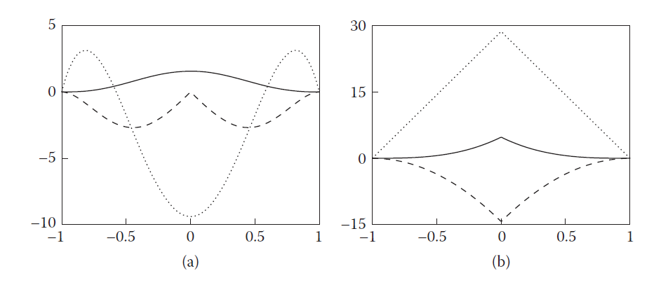
  但是，当我们需要求取核函数的梯度向量核拉普拉斯算子的时候，我们并不会采用poly6核函数，这是因为虽然其原函数很光滑，但其一阶导数和二阶导数的性质却不是很好，因而不会使用poly6的导数。对于梯度向量和拉普拉斯的求取，我们用spiky核函数取而代之：

$$W_{poly6}(r,h)=\frac{15}{\pi h^3} \begin{cases} (1-\frac{r}{h})^3\ \ 0\leq r\leq h\\ 0\ \ \ \ \ \ \ \ \ \ \ \ \ \ \ otherwise \end{cases} \tag {15}$$

  下面的图2是关于poly6核函数与spiky核函数的函数曲线、一阶导数曲线和二阶导数曲线，左图是poly6函数的，右图是spiky函数的，实心曲线为函数自身的曲线，点线是函数的二阶导数曲线，而虚线则是函数的一阶导数曲线。可以看到poly6的一阶导数和二阶导数呈现出一个波动的形态，在中心处一阶导数甚至降为零。我们需要计算流体的压力梯度来确保流体的不可压缩性，如果直接采用poly6的一阶导数来计算流体的压力梯度力，那么当两个粒子重合时，其压力梯度力为零，不存在一个力使它们分开，从而违背了流体的不可压缩性。二阶导数同理，其甚至在中心处取值为负，二阶导数将用于拉普拉斯算子的计算，而流体的粘性力计算将用到拉普拉斯算子。

图2 poly6和spiky的原函数、一阶导数和二阶导数比较

  spiky函数的一阶导数为：

$$\nabla W_{spiky}(r,h)=-\frac{45}{\pi h^4}(1-\frac{r}{h})^2 \tag {16}$$

inline double SphSpikyKernel3::firstDerivative(double distance) const 
{
	if (distance >= h) 
		return 0.0;
	else 
	{
		double x = 1.0 - distance / h;
		return -45.0 / (kPiD * h4) * x * x;
	}
}

inline Vector3D SphSpikyKernel3::gradient(const Vector3D& point) const 
{
	double dist = point.length();
	if (dist > 0.0) 
		return gradient(dist, point / dist);
	else 
		return Vector3D(0, 0, 0);
}

inline Vector3D SphSpikyKernel3::gradient(double distance, const Vector3D& directionToCenter) const 
{
	return -firstDerivative(distance) * directionToCenter;
}

  spiky函数的二阶导数为：

$$\nabla^2 W_{spiky}(r,h)=\frac{90}{\pi h^5}(1-\frac{r}{h}) \tag {17}$$

inline double SphSpikyKernel3::secondDerivative(double distance) const 
{
	if (distance >= h) 
		return 0.0;
	else 
	{
		double x = 1.0 - distance / h;
		return 90.0 / (kPiD * h5) * x;
	}
}

二、SPH流体模拟算法

  首先是简化的Naiver-Stokes方程，分为两部分，分别是动量方程$(18)$和连续方程$(19)$：

$$\frac{D \vec v}{D t}=-\frac{1}{\rho}\nabla p+\mu \nabla^2 \vec v+\vec g \tag {18}$$ $$\frac{\partial \rho}{\partial t}+\nabla \cdot (\rho \vec v) = 0 \tag {19}$$

  连续方程描述了流体的密度随着时间的变化速率，我们的模拟的是不可压缩流体，因而密度守恒，故$\frac{\partial \rho}{\partial t}=0$，即$\nabla \cdot \vec v=0$，流体的速度场满足无散度的条件。动量方程左边的是速度关于时间的物质导数，$\frac{D\vec v}{D t}=\frac{\partial \vec v}{\partial t}+\vec v\cdot \nabla \vec v$。在我们的基于粒子的流体模拟算法中，质量守恒自动满足，$\vec v\cdot \nabla \vec v=0$，粒子速度场关于时间的物质导数就是$\frac{\partial \vec v}{\partial t}$。上述公式中的$\vec g$是重力加速度，$\mu$是流体的黏度系数，$\rho$是流体密度，$p$是流体压强。

  每一个粒子的加速度为：

$$a=-\frac{1}{\rho}\nabla p+\mu \nabla^2\vec v+\vec g \tag {20}$$

  在公式$(20)$的右边分别是流体的压力项$-\frac{1}{\rho}\nabla p$、粘性力项$\mu \nabla^2\vec v$以及体积力项$\vec g$（在这里目前只有重力）。在模拟的过程中，我们需要分别计算这几项。一个完整的SPH流体求解器计算流程如下所示：

1.Measure the density with particles’ current locations
2.Compute the gravity and other extra forces
3.Compute the viscosity force
4.Compute the pressure based on the density
5.Compute the pressure gradient force
6.Perform time integration

  接下来按照这个步骤一一展开。

1、计算粒子的密度

  首先我们要计算流体粒子的密度值，因为后面粘性力和压强梯度力的计算将会用到粒子的密度。粒子的密度同样是采用光滑核对周围粒子进行加权计算，将密度函数代入公式$(4)$,

$$\begin{align} f(x)\approx & \Sigma_{i=1}^N \frac{m_i}{\rho_i}\rho_i w(||x-x_i||/h_i)\\ \approx & \Sigma_{i=1}^Nm_i w(||x-x_i||/h_i) \end{align} \tag {21}$$

  原公式中的密度项被消去了，所以我们直接根据粒子的位置和质量计算每个粒子的密度，在这里我们的每个粒子质量都相同：

void SphSystemData3::updateDensities() 
{
	auto p = positions();
	auto d = densities();
	const double m = mass();

	parallelFor(kZeroSize, numberOfParticles(), [&](size_t i) {
		double sum = sumOfKernelNearby(p[i]);
		d[i] = m * sum;
	});
}

double SphSystemData3::sumOfKernelNearby(const Vector3D& origin) const 
{
	double sum = 0.0;
	SphStdKernel3 kernel(_kernelRadius);
	neighborSearcher()->forEachNearbyPoint(
		origin, _kernelRadius, [&](size_t, const Vector3D& neighborPosition) {
		double dist = origin.distanceTo(neighborPosition);
		sum += kernel(dist);
	});
	return sum;
}

2、计算外部作用力

  这里指的外部的作用力通常是体积力，即间接地作用在流体上而非通过直接接触产生的作用力。常见的体积力有重力和风力，这些体积力我们直接根据需要指定其加速度的值，然后采用牛顿定律叠加到粒子的力场上：

void ParticleSystemSolver3::accumulateExternalForces() 
{
	size_t n = _particleSystemData->numberOfParticles();
	auto forces = _particleSystemData->forces();
	auto velocities = _particleSystemData->velocities();
	auto positions = _particleSystemData->positions();
	const double mass = _particleSystemData->mass();
	parallelFor(kZeroSize, n,
		[&](size_t i)
	{
		// Gravity
		Vector3D force = mass * _gravity;
		// Wind
		Vector3D relativeVel = velocities[i] - _wind->sample(positions[i]);
		force += -_dragCoefficient * relativeVel;
		forces[i] += force;
	});
}

3、计算流体粘性力

  流体的粘性力是流体内部的一种阻力，粘性力的计算需要计算流体速度场的拉普拉斯算子，这是因为拉普拉斯算子衡量了给定位置的物理量与周围邻域物理量的差距值：

$$f_{v}=m\mu \nabla ^2\vec v \tag {22}$$

  在SPH的算法中，其同样是通过光滑核函数计算粘性力，注意这里为了避免常量函数的拉普拉斯算子为非零，采用了前面的公式$(8)$：

$$f_v(x)=m^2\mu\Sigma_j(\frac{\vec v_j-\vec v_i}{\rho_j})\nabla^2W(x-x_j) \tag {23}$$

void SphSolver3::accumulateViscosityForce() 
{
	auto particles = sphSystemData();
	size_t numberOfParticles = particles->numberOfParticles();
	auto x = particles->positions();
	auto v = particles->velocities();
	auto d = particles->densities();
	auto f = particles->forces();

	const double massSquared = square(particles->mass());
	const SphSpikyKernel3 kernel(particles->kernelRadius());

	parallelFor(kZeroSize, numberOfParticles,
		[&](size_t i) 
	{
		const auto& neighbors = particles->neighborLists()[i];
		for (size_t j : neighbors) 
		{
			double dist = x[i].distanceTo(x[j]);
			f[i] += viscosityCoefficient() * massSquared * (v[j] - v[i]) / d[j]
				* kernel.secondDerivative(dist);
		}
	});
}

4、计算流体的压强

  流体的压强是流体内部的一种力，它是维持流体不可压缩的关键。目前我们只知道流体的密度值，流体的密度与压强存在着某种联系，密度大的趋于压强必然大，因此需要根据流体的密度计算其对应的压强值。当然我们可以直接求解关于流体压强的泊松方程$\nabla ^2P=\rho \frac{\nabla \vec v}{\Delta t}$，这样求解得到的压强是非常精确的，直接求解泊松方程在基于欧拉网格的流体模拟中比较常见，但是求解大规模稀疏矩阵的泊松方程非常耗时，因此在基于拉格朗日粒子的流体模拟中比较少（但也有），一种非常廉价且效果非常不错的方法就是采用泰特的状态方程：

$$P=B((\frac{\rho}{\rho_0})^\gamma -1) \tag {24}$$

  公式$(24)$中，$\rho_0$流体静止时的密度，$\rho$是流体粒子当前的密度，$\gamma$是状态方程的指数，取值为$7$，而$B$则是一个缩放系数因子，与声波在流体中的传播速度有关，其计算公式如下：

$$B=\frac{\rho_0 c_s^2}{\gamma} \tag {25}$$

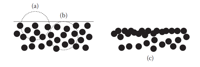
  通过这个状态方程，我们可以计算出流体的压强值。但是存在一个问题，对于的粒子密度，我们是通过邻域粒子来计算的，这意味着流体表面的粒子因为邻域粒子较少使得其计算出来的密度值$\rho$低于静止时的密度$\rho_0$，导致通过状态方程计算出来的压强为负数，如下图3所示，从而导致流体在表面上的不正常聚集现象，这种现象类似于表面张力，但它并不是物理意义上准确的，所以我们需要消除这种现象。当计算得到的压强为负时，我们赋予为零。

图3 表面的低密度导致的负压强使粒子不正常地聚集

double SphSolver3::computePressureFromEos(
	double density,
	double targetDensity,
	double eosScale,
	double eosExponent, 
	double negativePressureScale)
{
	double p = eosScale *
		(std::pow((density / targetDensity), eosExponent) - 1.0);

	// Negative pressure Scaling.
	if (p < 0)
		p *= negativePressureScale;

	return p;
}

void SphSolver3::computePressure()
{
	auto particles = sphSystemData();
	size_t numberOfParticles = particles->numberOfParticles();
	auto d = particles->densities();
	auto p = particles->pressures();

	// See Equation 9 from
	// http://cg.informatik.uni-freiburg.de/publications/2007_SCA_SPH.pdf
	const double targetDensity = particles->targetDensity();
	const double eosScale = targetDensity * square(_speedOfSound) / _eosExponent;

	parallelFor(kZeroSize, numberOfParticles,
		[&](size_t i)
	{
		p[i] = computePressureFromEos(
			d[i],
			targetDensity,
			eosScale,
			eosExponent(),
			negativePressureScale());
	});
}

5、计算压强梯度力

  前面一步我们得到了流体粒子的压强，在压强的作用下，流体粒子从高压强区域流向低压强区域，是流体保持不可压缩的性质。因此，我们需要计算作用在流体粒子上的压强梯度力项，压力梯度力计算公式为：

$$f_p=-m\frac{\nabla p}{\rho} \tag {26}$$

  利用前面的核函数拉普拉斯算子计算公式$(11)$，压强梯度力离散计算公式为：

$$f_p=-m^2\Sigma_j(\frac{p_i}{\rho_i^2}+\frac{p_j}{\rho_j^2})\nabla W(x-x_j) \tag {27}$$

void SphSolver3::accumulatePressureForce(
	const ConstArrayAccessor1<Vector3D>& positions,
	const ConstArrayAccessor1<double>& densities,
	const ConstArrayAccessor1<double>& pressures,
	ArrayAccessor1<Vector3D> pressureForces)
{
	auto particles = sphSystemData();
	size_t numberOfParticles = particles->numberOfParticles();

	const double massSquared = square(particles->mass());
	const SphSpikyKernel3 kernel(particles->kernelRadius());

	parallelFor(kZeroSize, numberOfParticles,
		[&](size_t i)
	{
		const auto& neighbors = particles->neighborLists()[i];
		for (size_t j : neighbors) 
		{
			double dist = positions[i].distanceTo(positions[j]);
			if (dist > 0.0) 
			{
				Vector3D dir = (positions[j] - positions[i]) / dist;
				pressureForces[i] -= massSquared
					* (pressures[i] / (densities[i] * densities[i]) + pressures[j] / (densities[j] * densities[j]))
					* kernel.gradient(dist, dir);
			}
		}
	});
}

6、时间步进积分

  前面我们计算得到每个流体粒子的作用力合力，接着需要根据这个力计算粒子的加速度，然后在加速度的作用下更新粒子的速度值，最后在速度的作用下计算粒子的位置向量。这个步骤只需简单地利用牛顿定律即可。

void ParticleSystemSolver3::timeIntegration(double timeStepInSeconds) 
{
	size_t n = _particleSystemData->numberOfParticles();
	auto forces = _particleSystemData->forces();
	auto velocities = _particleSystemData->velocities();
	auto positions = _particleSystemData->positions();
	const double mass = _particleSystemData->mass();
	parallelFor(kZeroSize, n,
		[&](size_t i) {
		// Integrate velocity first
		Vector3D& newVelocity = _newVelocities[i];
		newVelocity = velocities[i]
			+ timeStepInSeconds * forces[i] / mass;
		// Integrate position.
		Vector3D& newPosition = _newPositions[i];
		newPosition = positions[i] + timeStepInSeconds * newVelocity;
	});
}

7、碰撞检测处理

  在获取了新得速度场和位置向量之后，我们需要做碰撞检测处理，使之不发生穿透。这里的碰撞检测采用了隐式表面的符号距离场，为每个碰撞体构建一个水平集，这方面的内容比较多，但不是这里的核心点，故不赘述。目前实现的是刚体碰撞。下面只是一部分代码。

void Collider3::resolveCollision(
	double radius,
	double restitutionCoefficient,
	Vector3D* newPosition,
	Vector3D* newVelocity) 
{
	assert(_surface);

	if (!_surface->isValidGeometry()) 
		return;

	ColliderQueryResult colliderPoint;

	getClosestPoint(_surface, *newPosition, &colliderPoint);

	// Check if the new position is penetrating the surface
	if (isPenetrating(colliderPoint, *newPosition, radius)) 
	{
		// Target point is the closest non-penetrating position from the
		// new position.
		Vector3D targetNormal = colliderPoint.normal;
		Vector3D targetPoint = colliderPoint.point + radius * targetNormal;
		Vector3D colliderVelAtTargetPoint = colliderPoint.velocity;

		// Get new candidate relative velocity from the target point.
		Vector3D relativeVel = *newVelocity - colliderVelAtTargetPoint;
		double normalDotRelativeVel = targetNormal.dot(relativeVel);
		Vector3D relativeVelN = normalDotRelativeVel * targetNormal;
		Vector3D relativeVelT = relativeVel - relativeVelN;

		// Check if the velocity is facing opposite direction of the surface
		// normal
		if (normalDotRelativeVel < 0.0) 
		{
			// Apply restitution coefficient to the surface normal component of
			// the velocity
			Vector3D deltaRelativeVelN = (-restitutionCoefficient - 1.0) * relativeVelN;
			relativeVelN *= -restitutionCoefficient;

			// Apply friction to the tangential component of the velocity
			// From Bridson et al., Robust Treatment of Collisions, Contact and
			// Friction for Cloth Animation, 2002
			// http://graphics.stanford.edu/papers/cloth-sig02/cloth.pdf
			if (relativeVelT.lengthSquared() > 0.0) 
			{
				double frictionScale = std::max(1.0 - _frictionCoeffient * deltaRelativeVelN.length() /
					relativeVelT.length(), 0.0);
				relativeVelT *= frictionScale;
			}

			// Reassemble the components
			*newVelocity = relativeVelN + relativeVelT + colliderVelAtTargetPoint;
		}

		// Geometric fix
		*newPosition = targetPoint;
	}
}

void ParticleSystemSolver3::resolveCollision(
	ArrayAccessor1<Vector3D> newPositions,
	ArrayAccessor1<Vector3D> newVelocities) 
{
	if (_collider != nullptr) 
	{
		size_t numberOfParticles = _particleSystemData->numberOfParticles();
		const double radius = _particleSystemData->radius();

		parallelFor(kZeroSize, numberOfParticles,
			[&](size_t i) {
			_collider->resolveCollision(
				radius,
				_restitutionCoefficient,
				&newPositions[i],
				&newVelocities[i]);
		});
	}
}

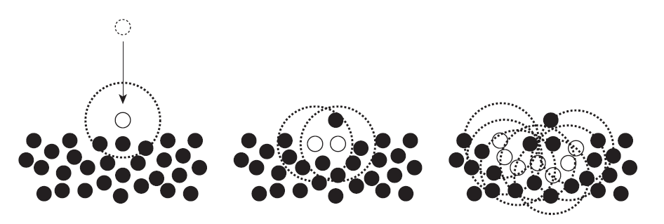
8、自适应时间步长

  最后还有个非常关键的点，就是模拟的时间步长选取。为了使得流体的密度守恒（即保持不可压缩性），我们采用了泰特的状态方程，该方程引入了两个参数，分别是指数$\gamma$和声波在流体中的传播速度，这带来了一些时间步长的限制问题。如下图4所示，假设一个流体粒子从空中落到一滩流体中，这个过程会产生一些震荡波，白色的粒子是落下的粒子以及获取到了震荡波动信息的粒子。

图4 流体粒子的信息传播

  受限于有限的光滑核半径，在每一个时间步长内，信息传播的范围最大为光滑核半径的长度。设信息的传播速度为$c$，那么我们能取得最大时间步长就为$h/c$。在我们得物理模拟中，这个信息传播速度实际上就是声波在流体中的传播速度。为此，研究者们提出自适应的时间步长，根据当前的流体状态计算最大的时间步长，如果取超过这个最大时间步长限制，那么将会导致流体崩溃，产生不稳定的问题。时间步长的上界计算公式为：

$$\begin{align} &\Delta t_v=\frac{\lambda_v h}{c_s}\\ &\Delta t_f=\lambda_f \sqrt{\frac{mh}{F_{max}}}\\ &\Delta t\leq min(\Delta t_v, \Delta t_f) \end{align} \tag {28}$$

  其中，$h$是光滑核半径，$m$粒子质量，$c_s$是声波在流体中的传播速度，$F_{max}$是流体粒子当中受到的最大合力的长度值，$\lambda_v$和$\lambda_f$是一个缩放系数，分别取$0.4$和$0.25$。可以看到，时间步长的上界不仅仅取决于声波的传播速度，还取决于每一个不同的时刻流体所受的最大合力，因而每一次模拟都要重新计算下一个时间步长。

unsigned int SphSolver3::numberOfSubTimeSteps(double timeIntervalInSeconds) const 
{
	auto particles = sphSystemData();
	size_t numberOfParticles = particles->numberOfParticles();
	auto f = particles->forces();

	const double kernelRadius = particles->kernelRadius();
	const double mass = particles->mass();

	double maxForceMagnitude = 0.0;

	for (size_t i = 0; i < numberOfParticles; ++i) 
		maxForceMagnitude = std::max(maxForceMagnitude, f[i].length());

	double timeStepLimitBySpeed = kTimeStepLimitBySpeedFactor * kernelRadius / _speedOfSound;
	double timeStepLimitByForce = kTimeStepLimitByForceFactor * std::sqrt(kernelRadius * mass / maxForceMagnitude);

	double desiredTimeStep = _timeStepLimitScale * std::min(timeStepLimitBySpeed, timeStepLimitByForce);

	return static_cast<unsigned int>(std::ceil(timeIntervalInSeconds / desiredTimeStep));
}

  真实世界中的声波在流体中的传播速度很快，这导致通过公式$(28)$计算得到的时间步长是非常小的。举个例子，假设我们的光滑核半径为$0.1m$，质量为$0.01kg$，声波传播速度为$1482m/s$，在只有重力这个外力的作用下，根据公式$(28)$计算可得$\Delta t_v=0.00002699055331s$，而$\Delta t_f=0.0007985957062$，因此最大的时间步长为$0.00002699055331$，这意味着如果模拟$60$帧率的话，那么一秒需要计算$618$个子时间步长，耗费大量的时间和计算资源，即便是离线模拟，其代价也太大了。这个就是传统的SPH算法的缺点，被称为WCSPH（Weakly Compressible SPH），针对这个缺点，目前已经有不少研究者提出了不同的改进方法，其中比较优秀的算法就是PCISPH。

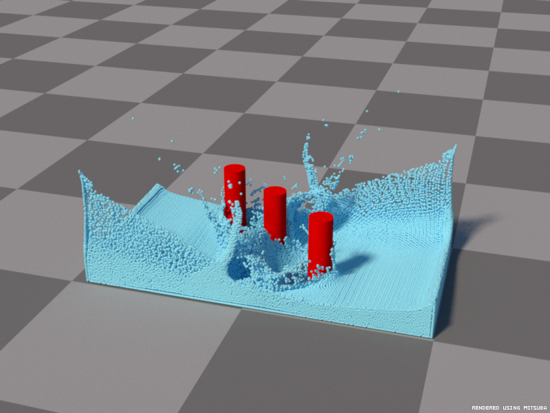
9、模拟效果

  整个模拟系统比较大，关于粒子数据的结构、邻域搜索算法、多线程并行、系统结构等方面不再赘述。我们模拟的结果是粒子群的位置向量，为了渲染出来需要采用一个算法根据粒子点云提取流体表面的三角网格，通常的流程就是根据粒子点云计算一个水平集，关于这方面目前已经不少学者研究并提出了几种算法，目前先采用最简单的一种提取表面算法，以后再回过头来查看这方面的算法。提取出来的表面之后采用了一个Mitsuba光追渲染器，模拟并渲染了两个场景，一个是Fluid Drop场景，一个是Dam Breaking场景。

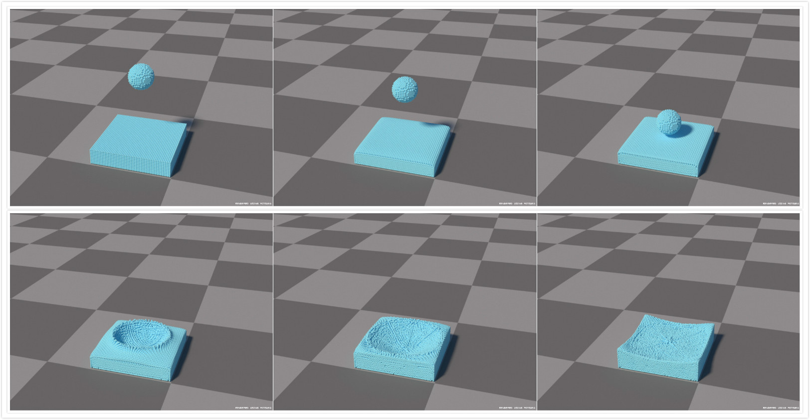
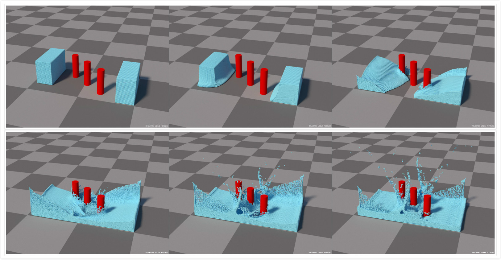
  由于传统的SPH模拟太过耗时，所以我就没有提取出流体的表面了，而是直接渲染流体的粒子。后面采用了改进的算法再提取流体表面，渲染极度真实的流体。下面的图5和图6分别展示了Fluid Drop场景和Dam Breaking场景的第0、10、20、30、40、50帧的流体粒子渲染结果。

图5 Fluid Drop的第0、10、20、30、40、50帧

图6 Dam Breaking的第0、10、20、30、40、50帧

三、PCISPH流体模拟算法

  传统的SPH算法采用了泰特的状态方程来计算流体压强，避免了求解大型稀疏矩阵的泊松方程，但是受限于状态方程中的声波速度，我们不能取太大的刚度系数，否则将导致时间步长非常小，极大地耗费计算资源。因此，后来又有学者提出了传统SPH算法的改进——PCISPH（全称为Predictive-Corrective Incompressible SPH，译为预测-矫正的不可压缩SPH，简称PCISPH）。与WCSPH算法不同，PCISPH不再采用泰特方程来计算流体的压强值，而是采用了一种非线性的迭代方法，尽可能地计算一个使得流体密度守恒的压强值。

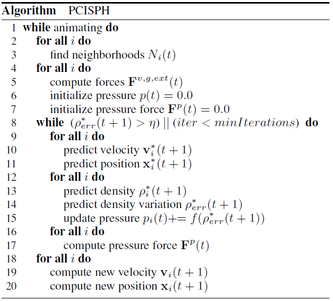
  PCISPH总体算法如下图7所示。可以看到，在求解流体的压强梯度力时，它是一个循环迭代的过程，迭代的终止条件为流体的当前密度与静止密度之差小于给定的阈值或者达到最大的迭代次数。

图7 PCISPH算法纵览

  在每一重迭代的过程种，首先根据粒子的净合力计算加速度，并计算在当前加速度下的速度值、位置向量，这一过程称为预测过程。紧接着计算前面预测得到的粒子群的密度值以及当前的密度值与静止密度的差距，并根据这个密度差计算压强，使得在这个压强的作用下，我们的粒子能够移动到一个位置上从而缩小这个密度差距。最后根据压强计算压强梯度力，将其迭代到我们的合力当中，用以下一次的迭代。

  迭代过程的关键一步就是如何根据密度差计算出所需的压强值，这涉及到一些数学内容。设光滑核半径长度为$h$，给定一点$i$在第$t+1$时间点的密度值通过下面的公式计算得到：

$$\begin{align} \rho_i(t+1)&= m\Sigma_j W(x_i(t+1)-x_j(t+1))\\ &= m\Sigma_jW(x_i(t)+\Delta x_i(t)-x_j(t)-\Delta x_j(t))\\ &= m\Sigma_jW(d_{ij}(t)+\Delta d_{ij}(t)) \end{align} \tag {29}$$

  其中$d_{ij}(t)=x_i(t)-x_j(t)$，$\Delta d_{ij}(t)=\Delta x_i(t)-\Delta x_j(t)$。假设$\Delta d_{ij}$足够小，对$W(d_{ij}(t)+\Delta d_{ij}(t))$做一阶泰勒展开：

$$\begin{align} \rho_i(t+1) &= m\Sigma_j[W(d_{ij}(t))+\nabla W(d_{ij}(t))\cdot \Delta d_{ij}(t)]\\ &= m\Sigma_j W(x_i(t)-x_j(t))+m\Sigma_j \nabla W(x_i(t)-x_j(t))\cdot(\Delta x_i(t)- \Delta x_j(t))\\ &= \rho_i(t)+\Delta \rho_i(t) \end{align} \tag {30}$$

  上式中，$\Delta \rho_i(t)$是未知项，我们对其做一些展开：

$$\begin{align} \Delta \rho_i(t) &=m\Sigma_j\nabla W_{ij}\cdot (\Delta x_i(t)-\Delta x_j(t))\\ &=m(\Sigma_j \nabla W_{ij}\Delta x_i(t)-\Sigma_j\nabla W_{ij}\Delta x_j(t))\\ &=m(\Delta x_i(t)\Sigma_j \nabla W_{ij}-\Sigma_j \nabla W_{ij}\Delta x_j(t)) \end{align} \tag {31}$$

  令$\Delta x_i$为在仅仅考虑流体压强梯度力的情况下的位移向量，则有：

$$\Delta x_i=\Delta t^2\frac{F_i^p}{m} \tag {32}$$

  在理想的情况下，我们的流体应该处于一种这样的平衡状态：流体粒子的压强值均等于$\overline p_i$，流体粒子的密度值均为静止时的密度$\rho_0$，即有：

$$F_i^p=-m^2\Sigma_j(\frac{\overline p_i}{\rho_0^2}+\frac{\overline p_i}{\rho_0^2})\nabla W_{ij}=-m^2\frac{2\overline p_i}{\rho_0^2}\Sigma_j \nabla W_{ij} \tag {33}$$

  将公式$(33)$代入公式$(32)$，可得：

$$\Delta x_i=-\Delta t^2 m\frac{2\overline p_i}{\rho_0^2}\Sigma_j\nabla W_{ij} \tag {34}$$

  记在粒子$i$的压强作用下，邻域粒子$j$的位移为$\Delta x_{j|i}$，因力是相互作用、相互对称的，则粒子$j$受到来自$i$的压强梯度力为：

$$F_{j|i}^p=m^2(\frac{\overline p_i}{\rho_0^2}+\frac{\overline p_i}{\rho_0^2}) \nabla W_{ij}=m^2\frac{2\overline p_i}{\rho_0^2}\nabla W_{ij} \tag {35}$$

  在上述的压强梯度力作用下：

$$\Delta x_{j|i}=\Delta t^2m\frac{2\overline p_i}{\rho_0^2}\nabla W_{ij} \tag {36}$$

  公式$(34)$和公式$(36)$给出了$\Delta x_i$和$\Delta x_{j|i}$，将其代入公式$(31)$中，得到了$\Delta \rho_i(t)$项的表达式：

$$\begin{align} \Delta \rho_i(t) &=m(-\Delta t^2m\frac{2\overline p_i}{\rho_0^2}\Sigma_j \nabla W_{ij}\cdot \Sigma_j \nabla W_{ij}-\Sigma_j(\nabla W_{ij}\cdot \Delta t^2 m\frac{2\overline p_i}{\rho_0^2}\nabla W_{ij}))\\ &=\Delta t^2m^2\frac{2\overline p_i}{\rho_0^2}(-\Sigma_j \nabla W_{ij}\cdot \Sigma_j \nabla W_{ij}-\Sigma_j(\nabla W_{ij}\cdot \nabla W_{ij})) \end{align} \tag {37}$$

  对公式$(37)$做一些变化，可得关于$\overline p_i$的一个表达式：

$$\overline p_i=\frac{\Delta \rho_i(t)} {\beta (-\Sigma_j\nabla W_{ij}\cdot \Sigma_j\nabla W_{ij}-\Sigma_j(\nabla W_{ij}\cdot \nabla W_{ij}))}\\ \beta=\Delta t^2m^2\frac{2}{\rho_0^2} \tag {38}$$

  而$\Delta \rho_i(t)=-\rho_{err_i}^t=-(\rho_i^t-\rho_0)$，即当前粒子的密度值与静止密度的差。公式$(38)$中的系数可以提出来提前计算，即下面的公式$(39)$，一方面是为了性能考虑，另一方面是因为表面粒子的邻域粒子数量少，其计算的系数是错的。

$$\delta =\frac{-1}{\beta(-\Sigma_j\nabla W_{ij}\cdot \Sigma_j\nabla W_{ij}-\Sigma_j(\nabla W_{ij}\cdot \nabla W_{ij}))} \tag {39}$$

double PciSphSolver3::computeBeta(double timeStepInSeconds) 
{
	auto particles = sphSystemData();
	return 2.0 * square(particles->mass() * timeStepInSeconds / particles->targetDensity());
}

double PciSphSolver3::computeDelta(double timeStepInSeconds)
{
	auto particles = sphSystemData();
	const double kernelRadius = particles->kernelRadius();

	Array1<Vector3D> points;
	BccLatticePointGenerator pointsGenerator;
	Vector3D origin;
	BoundingBox3D sampleBound(origin, origin);
	sampleBound.expand(1.5 * kernelRadius);

	pointsGenerator.generate(sampleBound, particles->targetSpacing(), &points);

	SphSpikyKernel3 kernel(kernelRadius);

	double denom = 0;
	Vector3D denom1;
	double denom2 = 0;

	for (size_t i = 0; i < points.size(); ++i) 
	{
		const Vector3D& point = points[i];
		double distanceSquared = point.lengthSquared();

		if (distanceSquared < kernelRadius * kernelRadius) 
		{
			double distance = std::sqrt(distanceSquared);
			Vector3D direction = (distance > 0.0) ? point / distance : Vector3D();

			// grad(Wij)
			Vector3D gradWij = kernel.gradient(distance, direction);
			denom1 += gradWij;
			denom2 += gradWij.dot(gradWij);
		}
	}

	denom += -denom1.dot(denom1) - denom2;

	return (std::fabs(denom) > 0.0) ? -1 / (computeBeta(timeStepInSeconds) * denom) : 0;
}

  然后$\overline p_i=\delta \rho_{err_i}^t$，在每一次的迭代中更新粒子的压强，$p_i+=\overline p_i$。PCISPH算法与WCSPH算法的不同就在计算压强梯度力上，除了更新粒子的压强值，还要更新粒子的密度值，并根据粒子的预测位置计算压强梯度力，整个迭代的流程不难理解。迭代结束之后，需要将迭代得到的压强梯度力加到粒子的合力上。

void PciSphSolver3::accumulatePressureForce(double timeIntervalInSeconds) 
{
	auto particles = sphSystemData();
	const size_t numberOfParticles = particles->numberOfParticles();
	const double delta = computeDelta(timeIntervalInSeconds);
	const double targetDensity = particles->targetDensity();
	const double mass = particles->mass();

	auto p = particles->pressures();
	auto d = particles->densities();
	auto x = particles->positions();
	auto v = particles->velocities();
	auto f = particles->forces();

	// Predicted density ds
	Array1<double> ds(numberOfParticles, 0.0);

	SphStdKernel3 kernel(particles->kernelRadius());

	// Initialize buffers
	parallelFor(kZeroSize, numberOfParticles,
		[&](size_t i) 
	{
		p[i] = 0.0;
		_pressureForces[i] = Vector3D();
		_densityErrors[i] = 0.0;
		ds[i] = d[i];
	});

	unsigned int maxNumIter = 0;
	double maxDensityError;
	double densityErrorRatio = 0.0;

	for (unsigned int k = 0; k < _maxNumberOfIterations; ++k) 
	{
		// Predict velocity and position
		parallelFor(kZeroSize, numberOfParticles,
			[&](size_t i) 
		{
			_tempVelocities[i] = v[i] + timeIntervalInSeconds / mass * (f[i] + _pressureForces[i]);
			_tempPositions[i] = x[i] + timeIntervalInSeconds * _tempVelocities[i];
		});

		// Resolve collisions
		resolveCollision(_tempPositions.accessor(), _tempVelocities.accessor());

		// Compute pressure from density error
		parallelFor(kZeroSize, numberOfParticles,
			[&](size_t i) 
		{
			double weightSum = 0.0;
			const auto& neighbors = particles->neighborLists()[i];
			for (size_t j : neighbors) 
			{
				double dist = _tempPositions[j].distanceTo(_tempPositions[i]);
				weightSum += kernel(dist);
			}
			weightSum += kernel(0);

			double density = mass * weightSum;
			double densityError = (density - targetDensity);
			double pressure = delta * densityError;
			if (pressure < 0.0) 
			{
				pressure *= negativePressureScale();
				densityError *= negativePressureScale();
			}

			p[i] += pressure;
			ds[i] = density;
			_densityErrors[i] = densityError;
		});

		// Compute pressure gradient force
		_pressureForces.set(Vector3D());
		SphSolver3::accumulatePressureForce(x, ds.constAccessor(), p, _pressureForces.accessor());

		// Compute max density error
		maxDensityError = 0.0;
		for (size_t i = 0; i < numberOfParticles; ++i) 
			maxDensityError = absmax(maxDensityError, _densityErrors[i]);

		densityErrorRatio = maxDensityError / targetDensity;
		maxNumIter = k + 1;

		if (std::fabs(densityErrorRatio) < _maxDensityErrorRatio) 
			break;
	}

	std::cout << "Number of PCI iterations: " << maxNumIter << std::endl;
	std::cout << "Max density error after PCI iteration: " << maxDensityError << std::endl;
	if (std::fabs(densityErrorRatio) > _maxDensityErrorRatio) 
	{
		std::cout << "Max density error ratio is greater than the threshold!\n";
		std::cout << "Ratio: " << densityErrorRatio << " Threshold: " << _maxDensityErrorRatio << std::endl;
	}

	// Accumulate pressure force
	parallelFor(kZeroSize, numberOfParticles,
		[this, &f](size_t i) 
	{
		f[i] += _pressureForces[i];
	});
}

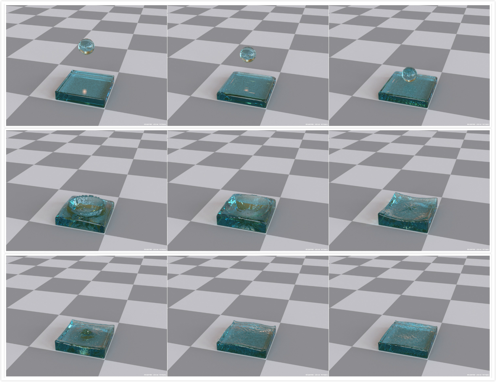
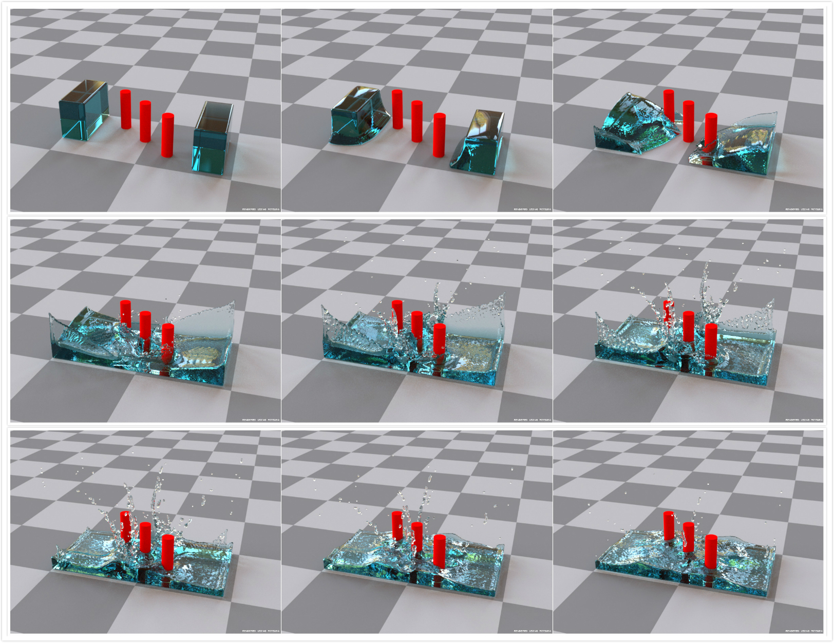
  与传统的WCSPH相比，PCISPH看起来步骤更多，因为它需要迭代多次，但是其不再依赖泰特方程，从而支持更大的时间步长，因此速度比WCSPH快很多。下图8和图9展示了Fluid Drop场景和Dam Breaking的场景模拟效果，采用了Marching Cubes重建流体表面进行渲染，效果与WCSPH几乎无差别，但是加速比起码有10倍以上，而且不可压缩性更好。这就是PCISPH算法的优势。

图8 Fluid Drop的第0、10、20、30、40、50、60、70、80帧

图9 Dam Breaking的第0、10、20、30、40、50、60、70、80帧

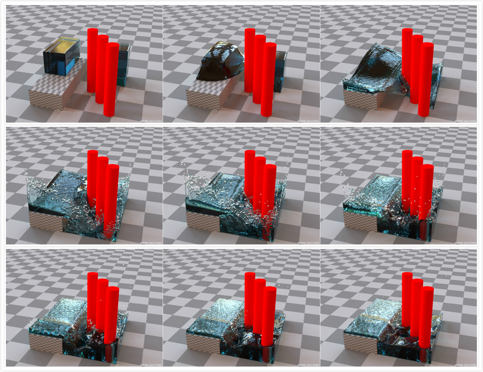
  最后，用PCISPH的流体求解算法模拟了一个稍微比较复杂的流体场景，模拟了600帧，不敢用WCSPH模拟600帧，因为WCSPH算法实在是太慢了。下图10展示了第0、20、40、60、80、100、120、140、160帧的效果。

图10 一个复杂场景的第0、20、40、60、80、100、120、140、160帧

参考资料：

$[1]$ Müller M, Charypar D, Gross M. Particle-based fluid simulation for interactive applications[C]//Proceedings of the 2003 ACM SIGGRAPH/Eurographics symposium on Computer animation. Eurographics Association, 2003: 154-159.

$[2]$ Becker M, Teschner M. Weakly compressible SPH for free surface flows[C]//Proceedings of the 2007 ACM SIGGRAPH/Eurographics symposium on Computer animation. Eurographics Association, 2007: 209-217.

$[3]$ Schechter H, Bridson R. Ghost SPH for animating water[J]. ACM Transactions on Graphics (TOG), 2012, 31(4): 61.

$[4]$ Kim, D. (2017). Fluid engine development. Boca Raton: Taylor & Francis, a CRC Press, Taylor & Francis Group.

$[5]$ Adams and Wicke, Meshless approximation methods and applications in physics based modeling and animation, Eurographics tutorials 2009.

$[6]$ Dan Koschier, Jan Bender. Smoothed Particle Hydrodynamics Techniques for the Physics Based Simulation of Fluids and Solids, Eurographics Tutorial 2019.

$[7]$ Solenthaler B, Pajarola R. Predictive-corrective incompressible SPH[C]// Acm Siggraph. 2009.