继之前实现了CPU端的PBF算法之后,我去学了CUDA编程模型,本文就是关于用CUDA实现PBF算法在GPU上高速地模拟。
基于GPU的空间哈希
基于CUDA的PBF流体模拟
程序结果
参考资料
基于CUDA的PBF流体模拟 一、基于GPU的空间哈希 在之前我们讨论了N-body的GPU并行实现,实际上这是一种比较极端的例子。在N-body系统中,每个粒子的都要与剩下的所有粒子计算两两之间的相互作用,这种相互作用通常有穿透力(如万有引力,称为体积力),无论远近、大小。但是在一些其他的物理模拟中,粒子只与周围邻近的粒子产生相互作用,如刚体、流体等,这时距离当前粒子比较远的其他粒子不会对当前的粒子产生任何的影响,因为刚体、流体之间的相互作用通常需要接触之后才产生(极端的例子不考虑,如万有引力,因为通常考虑的质量太小,万有引力几乎为0),所以我们没有必要采用N-body的方法逐个计算剩下的所有例子与当前粒子的物理作用,因为这会大大增加冗余计算。
对于流体、刚体、软体等的物理交互模拟,我们通常都是考虑的局部相互作用,这种局部相互作用要么就是接触才产生,要么就是随着距离的增大而迅速减小至消失。因此在这类的物理模拟中,我们需要采用一种快速的算法,该算法获取周围邻近的粒子,用以后续的物理模拟计算。这种算法就是空间哈希,在前面用CPU实现PBF时我们已经讨论过,它将整个空间做一个分割,每个粒子映射到一个空间数据结构,寻找邻域粒子时直接搜索周围空间的存储列表,算法复杂度只有$O(N)$。但是在GPU上实现该类算法稍微麻烦了点,因为GPU上的数据结构通常只有线性表,同时还要慎重考虑内存访问的开销等。
在GPU上实现该类算法有两种思路,先说说第一种方案。第一种方案是直接存储均匀分割的所有空间,为每个空间单元预先申请一个固定的大小的存储空间,这样需要提前申请固定大小的显卡内存空间,而且通常非常大,申请之后每个粒子计算哈希值索引,根据索引将其存储到对应的空间单元,由于流体和刚体通常是聚集的,因为这样将导致大部分的显卡内存空间都是空置状态,浪费了大量的显存空间,存储方式比较稀疏。
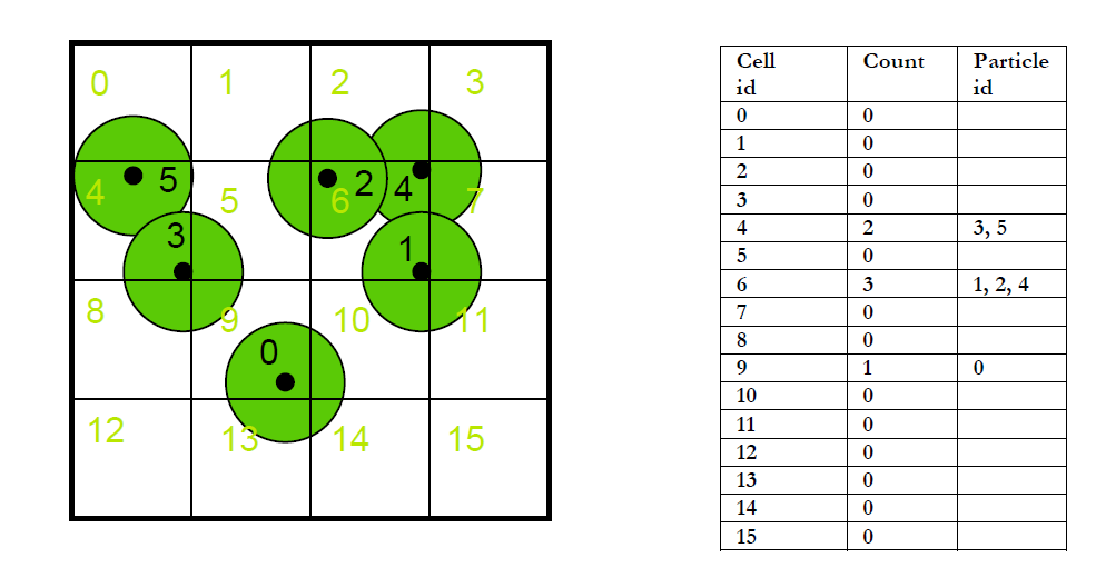
图1 方案一
如上图1的二维示例所示,方案一申请两个线性表,大小均为空间分割的分辨率,图中分割空间为$4\times 4=16$个。一个线性表为Count,记录当前的空间单元存在的粒子数目(为了避免写冲突,必须调用CUDA的原子操作指令atomicAdd),另外一个线性表记录每个空间单元中的粒子索引。当然我们也可以采用两个pass将粒子存储到一个连续的空间中,充分利用存储空间,但这需要两个pass,第一个pass计算每个空间单元的粒子数,然后第二个pass采用前缀和的方法计算每个空间单元存储的粒子的起始地址,最后将粒子连续地存储到线性表中。这个方法和接下来提到的采用排序的方法非常类似。
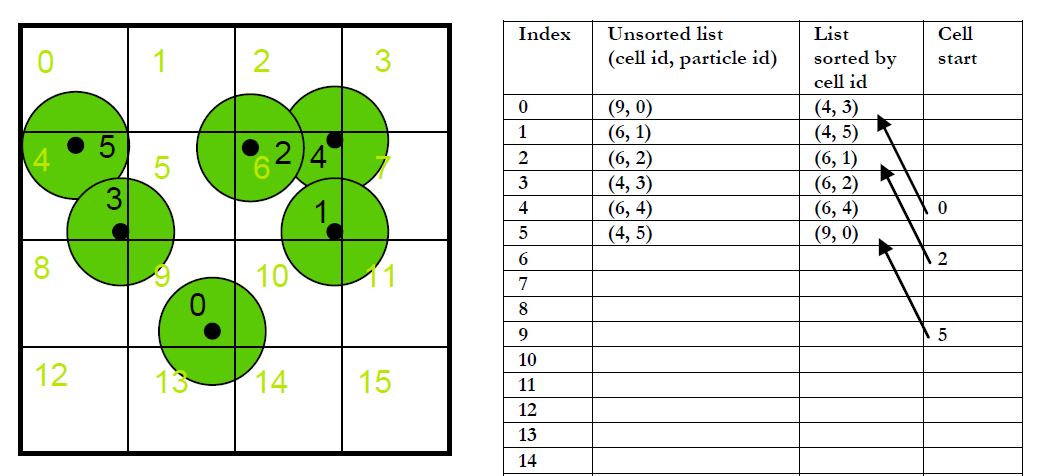
第二种方法采用排序将所有的粒子存储到紧凑的连续空间,节省大量的显存开销。如下图2所示,首先我们根据粒子的位置计算粒子的对应的空间哈希值,在这里我们目前只是简单地将粒子对应的线性编号作为它的哈希值cell id,然后将cell id和particle id这对数据存储线性数组中,其中我们要存储particle id是因为我们计算当前的cell id的时是根据粒子的位置来确定的,在后面我们需要用到这个对应关系,相当于一个索引。根据上面的步骤我们就得到了一个cell id乱序的线性表,接下来我们就根据这个cell id对整个数组做一个并行排序,使得数组的顺序是以cell id的顺序来排列的。这个过程相当于一个基数排序,因为一开始数组是以particle id为序的。得到这个以cell id为序的数组之后,我们需要记录每个空间单元cell记录的粒子起始地址和结束地址。判断起始地址很简单,只需将当前的cell id与数组的前一个cell id做比较,若不相同,则说明当前的粒子地址是当前粒子所在空间单元cell的起始地址,而且是其前一个粒子所在空间单元cell的终止地址。这样就能准确地记录每个空间单元的粒子。
图2 方案二
这里我们采用方案二的做法。首先需要计算每个粒子的空间hash值,前面已经说过,我们直接采用粒子的所在空间单元的线性编号,注意防止越界访问内存。下面的kernel代码calcGridPosKernel计算粒子所在空间单元的三维编号,接着calcGridHashKernel根据这个三维编号计算一维编号,最后将粒子索引id和哈希值存入两个对应的数组。
1
2
3
4
5
6
7
8
9
10
11
12
13
14
15
16
17
18
19
20
21
22
23
24
25
26
27
28
29
30
31
32
33
34
35
36
37
38
39
__device__ int3 calcGridPosKernel (float3 p) int3 gridPos; gridPos.x = floor ((p.x - params.m_worldOrigin.x) / params.m_cellSize.x); gridPos.y = floor ((p.y - params.m_worldOrigin.y) / params.m_cellSize.y); gridPos.z = floor ((p.z - params.m_worldOrigin.z) / params.m_cellSize.z); return gridPos; } __device__ unsigned int calcGridHashKernel (int3 gridPos) gridPos.x = gridPos.x & (params.m_gridSize.x - 1 ); gridPos.y = gridPos.y & (params.m_gridSize.y - 1 ); gridPos.z = gridPos.z & (params.m_gridSize.z - 1 ); return gridPos.z * params.m_gridSize.x * params.m_gridSize.y + gridPos.y * params.m_gridSize.x + gridPos.x; } __global__ void calcParticlesHashKernel ( unsigned int *gridParticleHash, unsigned int *gridParticleIndex, float4 *pos, unsigned int numParticles ) unsigned int index = blockIdx.x * blockDim.x + threadIdx.x; if (index >= numParticles) return ; volatile float4 curPos = pos[index]; int3 gridPos = calcGridPosKernel(make_float3(curPos.x, curPos.y, curPos.z)); unsigned int hashValue = calcGridHashKernel(gridPos); gridParticleHash[index] = hashValue; gridParticleIndex[index] = index; }
紧接着,我们需要对前面计算得到的两个数组做一个key-value排序,就是根据key的顺序来排列。同样为了效率,需要使用并行排序。CUDA提供了一个thrust库,直接调用库中的sort_by_key方法帮我们省去了这一个比较繁琐的工作。
1
2
3
4
5
6
7
8
9
10
11
void sortParticles ( unsigned int *deviceGridParticleHash, unsigned int *deviceGridParticleIndex, unsigned int numParticles ) thrust::sort_by_key( thrust::device_ptr<unsigned int >(deviceGridParticleHash), thrust::device_ptr<unsigned int >(deviceGridParticleHash + numParticles), thrust::device_ptr<unsigned int >(deviceGridParticleIndex)); }
前面对cell id和particle id排序之后,我们需要对存储粒子位置和速度属性的数组做一个相应的调整,使得其顺序与前面拍好的顺序一一对应。与此同时,还需要计算每个空间单元cell的起始地址和终止地址。这里我们充分利用同一个线程块的共享内存,设线程数有$n$个,那么我们申请$n+1$个单位大小的共享内存,每个线程首先将自己对应的那个粒子哈希值存储到共享内存中,第一个线程还要将其前一个粒子对应的哈希值存储到该共享内存中,这样可以避免每个线程访问全局内存2次(共2n次共享内存的访问),访问全局内存数变为了n+1次。然后每个粒子线程将当前对应的哈希值与其前一个粒子哈希值做比较,若不相同,则表明当前线程的index是空间单元cell的起始地址,终止地址同理。具体过程看如下的代码。我们设置cellStart初始为0xffffffff来表示它是一个空的cell单元,即没有任何的粒子落到该空间单元cell中。
1
2
3
4
5
6
7
8
9
10
11
12
13
14
15
16
17
18
19
20
21
22
23
24
25
26
27
28
29
30
31
32
33
34
35
36
37
38
39
40
41
42
43
44
45
46
47
48
49
50
51
52
53
54
55
56
57
58
59
60
61
62
63
64
65
66
67
68
69
70
71
72
73
74
75
76
77
78
79
80
__global__ void reoderDataAndFindCellRangeKernel ( unsigned int *cellStart, unsigned int *cellEnd, float4 *sortedPos, float4 *sortedVel, unsigned int *gridParticleHash, unsigned int *gridParticleIndex, float4 *oldPos, float4 *oldVel, unsigned int numParticles) thread_block cta = this_thread_block(); extern __shared__ unsigned int sharedHash[]; unsigned int index = blockIdx.x * blockDim.x + threadIdx.x; unsigned int hashValue; if (index < numParticles) { hashValue = gridParticleHash[index]; sharedHash[threadIdx.x + 1 ] = hashValue; if (index > 0 && threadIdx.x == 0 ) sharedHash[0 ] = gridParticleHash[index - 1 ]; } sync(cta); if (index < numParticles) { if (index == 0 || hashValue != sharedHash[threadIdx.x]) { cellStart[hashValue] = index; if (index > 0 ) cellEnd[sharedHash[threadIdx.x]] = index; } if (index == numParticles - 1 ) cellEnd[hashValue] = index + 1 ; unsigned int sortedIndex = gridParticleIndex[index]; float4 pos = oldPos[sortedIndex]; float4 vel = oldVel[sortedIndex]; sortedPos[index] = pos; sortedVel[index] = vel; } } void reorderDataAndFindCellRange ( unsigned int *cellStart, unsigned int *cellEnd, float *sortedPos, float *sortedVel, unsigned int *gridParticleHash, unsigned int *gridParticleIndex, float *oldPos, float *oldVel, unsigned int numParticles, unsigned int numCell) unsigned int numThreads, numBlocks; numThreads = 256 ; numBlocks = (numParticles % numThreads != 0 ) ? (numParticles / numThreads + 1 ) : (numParticles / numThreads); cudaMemset(cellStart, 0xffffffff , numCell * sizeof (unsigned int )); unsigned int memSize = sizeof (unsigned int ) * (numThreads + 1 ); reoderDataAndFindCellRangeKernel << <numBlocks, numThreads, memSize >> > ( cellStart, cellEnd, (float4*)sortedPos, (float4*)sortedVel, gridParticleHash, gridParticleIndex, (float4*)oldPos, (float4*)oldVel, numParticles); }
以上就是基于GPU的空间哈希过程,经过以上的步骤,粒子被紧凑地存储到线性空间,后面做物理计算时能快速地得到邻域空间的粒子。下面代码是整个基于GPU的空间哈希调用代码。
1 2 3 4 5 6 7 8 9 10 11 12 13 14 15 16 17 18 19 20 21 22 23 24 25 26 27 computeHash( m_deviceGridParticleHash, m_deviceGridParticleIndex, m_devicePos, m_params.m_numParticles ); sortParticles( m_deviceGridParticleHash, m_deviceGridParticleIndex, m_params.m_numParticles); reorderDataAndFindCellRange( m_deviceCellStart, m_deviceCellEnd, m_deviceSortedPos, m_deviceSortedVel, m_deviceGridParticleHash, m_deviceGridParticleIndex, m_devicePos, m_deviceVel, m_params.m_numParticles, m_params.m_numGridCells);
二、基于CUDA的PBF流体模拟 在之前我们实现了CPU的PBF流体模拟,受限于CPU的低并行度,我们只能实时模拟数量很少的流体粒子。为了能够快速模拟大量的粒子,我特意去学了CUDA,接下来就用CUDA实现之前讨论的PBF算法。暂时不用刚体粒子来实现流体碰撞边界。首先我们回顾一下之前提到的PBF(Position Based Fluid)算法,算法的伪代码如下所示。基于PBD的流体模拟算法大致可以分成几个部分:流体粒子对流、领域粒子搜索、不可压缩的压力约束投影、更新速度、涡轮修复、粘度计算以及最后的粒子位置更新。可以看到,第5行到第7行邻域粒子搜索的实现在本文的前面部分已经讨论过了,所以就不再赘述了。
在实现之前我们要弄清楚具体要申请多少的内存,仔细阅读上面的伪代码。首先我们必须申请两个位置向量数组,分别保存流体粒子的$x_i$和$x_i^*$。然后还需要一个数组存储粒子的位移信息$\Delta p_i$。最后需要存储粒子的速度信息,通常速度分量只需$(x,y,z)$即可,但是在算法的过程中还需要保存我们计算得到的拉格朗日乘子$\lambda_i$,所以我们申请分量为$(x,y,z,w)$的速度数组,第4个分量$w$存储拉格朗日乘子。
1、流体粒子对流 本部分即伪代码的第1行至第4行,在体积力(如重力)的作用下,粒子的速度场发生变换,进而导致粒子的位置发生变换。需要注意的是,我们目前采用的方法(即伪代码中的)是只有一阶精度的。计算得到的位置并不是立即替换掉当前的位置,需要保存一个新的数组中,因为最后我们需要根据旧的粒子位置和新的粒子位置计算粒子的速度场。
1
2
3
4
5
6
7
8
9
10
11
12
13
14
15
16
17
18
19
20
21
22
23
24
25
26
27
28
29
30
31
32
33
34
35
36
37
38
39
40
__global__ void advect ( float4 *position, float4 *velocity, float4 *predictedPos, float deltaTime, unsigned int numParticles) int index = blockIdx.x * blockDim.x + threadIdx.x; if (index >= numParticles) return ; float4 readVel = velocity[index]; float4 readPos = position[index]; float3 nVel; float3 nPos; nVel.x = readVel.x + deltaTime * params.m_gravity.x; nVel.y = readVel.y + deltaTime * params.m_gravity.y; nVel.z = readVel.z + deltaTime * params.m_gravity.z; nPos.x = readPos.x + deltaTime * nVel.x; nPos.y = readPos.y + deltaTime * nVel.y; nPos.z = readPos.z + deltaTime * nVel.z; if (nPos.x > 40.0f - params.m_particleRadius) nPos.x = 40.0f - params.m_particleRadius; if (nPos.x < params.m_leftWall + params.m_particleRadius) nPos.x = params.m_leftWall + params.m_particleRadius; if (nPos.y > 20.0f - params.m_particleRadius) nPos.y = 20.0f - params.m_particleRadius; if (nPos.y < -20.0f + params.m_particleRadius) nPos.y = -20.0f + params.m_particleRadius; if (nPos.z > 20.0f - params.m_particleRadius) nPos.z = 20.0f - params.m_particleRadius; if (nPos.z < -20.0f + params.m_particleRadius) nPos.z = -20.0f + params.m_particleRadius; predictedPos[index] = { nPos.x, nPos.y, nPos.z, readPos.w }; }
3、不可压缩约束投影 关于不可压缩的约束投影,具体在之前详细讲过,这里我们只是简单地回顾一下。首先PBF的不可压缩的密度约束公式如下所示,其中$\rho_i$是第$i$个粒子的密度值,$\rho_0$是流体静止时的密度值。
第$i$个流体粒子的密度计算我们采用SPH的方法,根据周围邻近粒子的质量做一个加权和,如下所示:
权重$W$函数我们采用Poly6核函数($h$是光滑核半径):
但是在计算密度的梯度时,我们又采用Spiky核函数:
Poly6核函数计算以及Spiky函数的梯度计算代码如下所示,为了性能,我提前在CPU端计算函数的常量系数:
1
2
3
4
5
6
7
8
9
10
11
12
13
14
15
16
17
18
19
20
21
22
23
24
25
__device__ float wPoly6 (const float3 &r) const float lengthSquared = r.x * r.x + r.y * r.y + r.z * r.z; if (lengthSquared > params.m_sphRadiusSquared || lengthSquared <= 0.00000001f ) return 0.0f ; float iterm = params.m_sphRadiusSquared - lengthSquared; return params.m_poly6Coff * iterm * iterm * iterm; } __device__ float3 wSpikyGrad (const float3 &r) const float lengthSquared = r.x * r.x + r.y * r.y + r.z * r.z; float3 ret = { 0.0f , 0.0f , 0.0f }; if (lengthSquared > params.m_sphRadiusSquared || lengthSquared <= 0.00000001f ) return ret; const float length = sqrtf(lengthSquared); float iterm = params.m_sphRadius - length; float coff = params.m_spikyGradCoff * iterm * iterm / length; ret.x = coff * r.x; ret.y = coff * r.y; ret.z = coff * r.z; return ret; }
然后公式$(1)$及其梯度就为:
拉格朗日乘子的计算公式就为:
这里我要重点强调的一点就是,流体静止时的密度设置很有必要思考一下。因为我假设粒子的质量都为$1kg$,所以公式中关于质量$m$的都可以直接去掉,我们需要根据流体粒子的体积计算静止时的密度。设一个粒子的半径为$r$,一个流体粒子当成立方体而不是球体,则其体积为$(2r)^3=8r^3$,那么静止时的密度$\rho_0=1/(8r^3)$,因为$\rho=m/v$。 接着我们根据公式$(2)$和公式$(6)$计算流体粒子的密度和拉格朗日乘子,并计算得到的拉格朗日乘子存储到速度的第四个分量上:
1
2
3
4
5
6
7
8
9
10
11
12
13
14
15
16
17
18
19
20
21
22
23
24
25
26
27
28
29
30
31
32
33
34
35
36
37
38
39
40
41
42
43
44
45
46
47
48
49
50
51
52
53
54
55
56
57
58
59
60
61
62
63
64
65
66
67
68
__global__ void calcLagrangeMultiplier ( float4 *predictedPos, float4 *velocity, unsigned int *cellStart, unsigned int *cellEnd, unsigned int *gridParticleHash, unsigned int numParticles, unsigned int numCells) int index = blockIdx.x * blockDim.x + threadIdx.x; if (index >= numParticles) return ; float4 readPos = predictedPos[index]; float4 readVel = velocity[index]; float3 curPos = { readPos.x, readPos.y, readPos.z }; int3 gridPos = calcGridPosKernel(curPos); float density = 0.0f ; float gradSquaredSum_j = 0.0f ; float gradSquaredSumTotal = 0.0f ; float3 curGrad, gradSum_i = { 0.0f ,0.0f ,0.0f }; #pragma unroll 3 for (int z = -1 ; z <= 1 ; ++z) { #pragma unroll 3 for (int y = -1 ; y <= 1 ; ++y) { #pragma unroll 3 for (int x = -1 ; x <= 1 ; ++x) { int3 neighbourGridPos = { gridPos.x + x, gridPos.y + y, gridPos.z + z }; unsigned int neighbourGridIndex = calcGridHashKernel(neighbourGridPos); unsigned int startIndex = cellStart[neighbourGridIndex]; if (startIndex == 0xffffffff ) continue ; unsigned int endIndex = cellEnd[neighbourGridIndex]; #pragma unroll 32 for (unsigned int i = startIndex; i < endIndex; ++i) { float4 neighbour = predictedPos[i]; float3 r = { curPos.x - neighbour.x, curPos.y - neighbour.y, curPos.z - neighbour.z }; density += wPoly6(r); curGrad = wSpikyGrad(r); curGrad.x *= params.m_invRestDensity; curGrad.y *= params.m_invRestDensity; curGrad.z *= params.m_invRestDensity; gradSum_i.x += curGrad.x; gradSum_i.y += curGrad.y; gradSum_i.z += curGrad.z; if (i != index) gradSquaredSum_j += (curGrad.x * curGrad.x + curGrad.y * curGrad.y + curGrad.z * curGrad.z); } } } } gradSquaredSumTotal = gradSquaredSum_j + gradSum_i.x * gradSum_i.x + gradSum_i.y * gradSum_i.y + gradSum_i.z * gradSum_i.z; float constraint = density * params.m_invRestDensity - 1.0f ; float lambda = -(constraint) / (gradSquaredSumTotal + params.m_lambdaEps); velocity[index] = { readVel.x, readVel.y, readVel.z, lambda }; }
计算完拉格朗日乘子之后,我们需要根据它来计算流体粒子的矫正位移量。同样,矫正偏移量的公式如下所示,同样我们考虑了邻近粒子的作用。
进一步地,为了防止粒子聚集导致流体表面失真,造成拉伸不稳定性,我们需要给上面的矫正位移公式$(7)$增加一个人工排斥力,当流体粒子距离过近时该排斥力会使它们分开,避免产生粒子聚集的现象。
上面的排斥项会使得流体粒子的密度稍微低于静态密度,从而产生类似于表面张力的效果,使得流体表面的的粒子分布均匀。通过这个排斥项,我们不再需要硬性规定流体的邻居数量必须在30~40个,进一步提升算法的流体模拟效率。根据公式$(8)$,我们计算矫正位移的cuda代码如下所示:
1
2
3
4
5
6
7
8
9
10
11
12
13
14
15
16
17
18
19
20
21
22
23
24
25
26
27
28
29
30
31
32
33
34
35
36
37
38
39
40
41
42
43
44
45
46
47
48
49
50
51
52
53
54
55
56
__global__ void calcDeltaPosition ( float4 *predictedPos, float4 *velocity, float3 *deltaPos, unsigned int *cellStart, unsigned int *cellEnd, unsigned int *gridParticleHash, unsigned int numParticles) int index = blockIdx.x * blockDim.x + threadIdx.x; if (index >= numParticles) return ; float4 readPos = predictedPos[index]; float4 readVel = velocity[index]; float3 curPos = { readPos.x, readPos.y, readPos.z }; int3 gridPos = calcGridPosKernel(curPos); float curLambda = readVel.w; float3 deltaP = { 0.0f , 0.0f , 0.0f }; #pragma unroll 3 for (int z = -1 ; z <= 1 ; ++z) { #pragma unroll 3 for (int y = -1 ; y <= 1 ; ++y) { #pragma unroll 3 for (int x = -1 ; x <= 1 ; ++x) { int3 neighbourGridPos = { gridPos.x + x, gridPos.y + y, gridPos.z + z }; unsigned int neighbourGridIndex = calcGridHashKernel(neighbourGridPos); unsigned int startIndex = cellStart[neighbourGridIndex]; if (startIndex == 0xffffffff ) continue ; unsigned int endIndex = cellEnd[neighbourGridIndex]; #pragma unroll 32 for (unsigned int i = startIndex; i < endIndex; ++i) { float4 neighbour = predictedPos[i]; float neighbourLambda = velocity[i].w; float3 r = { curPos.x - neighbour.x, curPos.y - neighbour.y, curPos.z - neighbour.z }; float corrTerm = wPoly6(r) * params.m_oneDivWPoly6; float coff = curLambda + neighbourLambda - 0.1f * corrTerm * corrTerm * corrTerm * corrTerm; float3 grad = wSpikyGrad(r); deltaP.x += coff * grad.x; deltaP.y += coff * grad.y; deltaP.z += coff * grad.z; } } } } float3 ret = {deltaP.x * params.m_invRestDensity, deltaP.y * params.m_invRestDensity, deltaP.z * params.m_invRestDensity }; deltaPos[index] = ret; }
最后,我们需要把前面计算得到的矫正位移加到位置向量上,从而使得粒子在移动之后依然保持流体不可压缩的特性。这里对应伪代码的第16行到第18行,比较简单。
1
2
3
4
5
6
7
8
9
10
11
12
13
14
15
16
17
__global__ void addDeltaPosition ( float4 *predictedPos, float3 *deltaPos, unsigned int numParticles) int index = blockIdx.x * blockDim.x + threadIdx.x; if (index >= numParticles) return ; float4 readPos = predictedPos[index]; float3 readDeltaPos = deltaPos[index]; readDeltaPos.x = readPos.x + readDeltaPos.x; readDeltaPos.y = readPos.y + readDeltaPos.y; readDeltaPos.z = readPos.z + readDeltaPos.z; predictedPos[index] = { readDeltaPos.x, readDeltaPos.y, readDeltaPos.z, readPos.w }; }
最后,约束投影并不是一次就够了,还需要迭代多次,我设置了迭代3次。
3、更新速度和位置 对应伪代码的第21行,我们根据流体粒子的上一帧位置和当前计算得到的位置计算粒子的速度值,直接根据速度的定义计算。这样计算到的速度将在下一帧产生作用,这也是Position Based Dynamics的由来,我们不是直接根据速度来更新粒子的位置,而是根据粒子的位移来更新粒子的速度,即“位置变化驱动”。最后将新的位置值覆盖到原先的位置向量上。
1
2
3
4
5
6
7
8
9
10
11
12
13
14
15
16
17
18
19
20
21
22
__global__ void updateVelocityAndPosition ( float4 *position, float4 *velocity, float4 *predictedPos, float invDeltaTime, unsigned int numParticles) int index = blockIdx.x * blockDim.x + threadIdx.x; if (index >= numParticles) return ; float4 oldPos = position[index]; float4 newPos = predictedPos[index]; float4 readVel = velocity[index]; float3 posDiff = { newPos.x - oldPos.x, newPos.y - oldPos.y, newPos.z - oldPos.z }; posDiff.x *= invDeltaTime; posDiff.y *= invDeltaTime; posDiff.z *= invDeltaTime; velocity[index] = { posDiff.x, posDiff.y, posDiff.z, readVel.w }; position[index] = { newPos.x, newPos.y, newPos.z, newPos.w }; }
4、涡轮修复和人工粘性 由于数值耗散,PBD的方法会引入额外的阻尼,使得整个系统的能量损耗太快,导致本来应该由的一些涡流细节迅速消失。在这里,PBF通过涡轮控制方法向整个系统重新注入能量($\epsilon$用于控制涡轮控制力的强度):
涡轮修复这一部分论文并未详细展开,然后我就按照自己的理解写了个大概,代码如下所示。结果发现还是有问题,暂先这样。
1
2
3
4
5
6
7
8
9
10
11
12
13
14
15
16
17
18
19
20
21
22
23
24
25
26
27
28
29
30
31
32
33
34
35
36
37
38
39
40
41
42
43
44
45
46
47
48
49
50
51
52
53
54
55
56
57
58
59
60
61
62
63
64
65
66
67
68
69
70
71
72
73
74
75
76
77
78
79
80
81
82
83
84
85
86
87
88
89
90
91
92
93
94
95
96
97
98
99
100
101
102
103
104
__global__ void calcVorticityConfinment ( float4 *velocity, float3 *deltaPos, float4 *predictedPos, unsigned int *cellStart, unsigned int *cellEnd, unsigned int *gridParticleHash, unsigned int numParticles) int index = blockIdx.x * blockDim.x + threadIdx.x; if (index >= numParticles) return ; float4 readPos = predictedPos[index]; float4 readVel = velocity[index]; float3 curPos = { readPos.x, readPos.y, readPos.z }; float3 curVel = { readVel.x, readVel.y, readVel.z }; int3 gridPos = calcGridPosKernel(curPos); float3 velDiff; float3 gradient; float3 omega = { 0.0f ,0.0f ,0.0f }; float3 eta = { 0.0f ,0.0f ,0.0f }; #pragma unroll 3 for (int z = -1 ; z <= 1 ; ++z) { #pragma unroll 3 for (int y = -1 ; y <= 1 ; ++y) { #pragma unroll 3 for (int x = -1 ; x <= 1 ; ++x) { int3 neighbourGridPos = { gridPos.x + x, gridPos.y + y, gridPos.z + z }; unsigned int neighbourGridIndex = calcGridHashKernel(neighbourGridPos); unsigned int startIndex = cellStart[neighbourGridIndex]; if (startIndex == 0xffffffff ) continue ; unsigned int endIndex = cellEnd[neighbourGridIndex]; #pragma unroll 32 for (unsigned int i = startIndex; i < endIndex; ++i) { float4 neighbourPos = predictedPos[i]; float4 neighbourVel = velocity[i]; velDiff = { neighbourVel.x - curVel.x, neighbourVel.y - curVel.y, neighbourVel.z - curVel.z }; gradient = wSpikyGrad({ curPos.x - neighbourPos.x, curPos.y - neighbourPos.y , curPos.z - neighbourPos.z }); float3 f = cross(velDiff, gradient); omega.x += f.x; omega.y += f.y; omega.z += f.z; eta.x += gradient.x; eta.y += gradient.y; eta.z += gradient.z; } } } } float omegaLength = sqrtf(omega.x * omega.x + omega.y * omega.y + omega.z * omega.z); float3 force = { 0.0f ,0.0f ,0.0f }; if (omegaLength == 0.0f ) { deltaPos[index] = force; return ; } eta.x *= omegaLength; eta.y *= omegaLength; eta.z *= omegaLength; if (eta.x == 0 && eta.y == 0 && eta.z == 0 ) { deltaPos[index] = force; return ; } float etaLength = sqrtf(eta.x * eta.x + eta.y * eta.y + eta.z * eta.z); eta.x /= etaLength; eta.y /= etaLength; eta.z /= etaLength; force = cross(eta, omega); force.x *= params.m_vorticity; force.y *= params.m_vorticity; force.z *= params.m_vorticity; deltaPos[index] = force; } __global__ void addVorticityConfinment ( float4 *velocity, float3 *deltaPos, float deltaTime, unsigned int numParticles) int index = blockIdx.x * blockDim.x + threadIdx.x; if (index >= numParticles) return ; float4 readVel = velocity[index]; float3 vorticity = deltaPos[index]; readVel.x += vorticity.x ; readVel.y += vorticity.y ; readVel.z += vorticity.z ; velocity[index] = readVel; }
最后,PBF方法采用XSPH的粘度方法直接更新速度,从而产生粘性阻尼。人工粘性除了可以增加模拟的数值稳定性,还可以消除非物理的流体振荡。拉格朗日流体模拟方法中,人工粘性本质上会对流体粒子的相对运动产生阻尼作用,使流体的动能转化为热能(同样目前我实现的有问题):
1
2
3
4
5
6
7
8
9
10
11
12
13
14
15
16
17
18
19
20
21
22
23
24
25
26
27
28
29
30
31
32
33
34
35
36
37
38
39
40
41
42
43
44
45
46
47
48
49
50
51
52
53
54
55
56
57
58
59
60
61
62
63
64
65
66
67
68
69
70
71
72
73
74
75
76
77
78
79
__global__ void calcXSPHViscosity ( float4 *velocity, float3 *deltaPos, float4 *predictedPos, unsigned int *cellStart, unsigned int *cellEnd, unsigned int *gridParticleHash, unsigned int numParticles) int index = blockIdx.x * blockDim.x + threadIdx.x; if (index >= numParticles) return ; float4 readPos = predictedPos[index]; float4 readVel = velocity[index]; float3 curPos = { readPos.x, readPos.y, readPos.z }; float3 curVel = { readVel.x, readVel.y, readVel.z }; int3 gridPos = calcGridPosKernel(curPos); float3 viscosity = { 0.0f ,0.0f ,0.0f }; float3 velocityDiff; #pragma unroll 3 for (int z = -1 ; z <= 1 ; ++z) { #pragma unroll 3 for (int y = -1 ; y <= 1 ; ++y) { #pragma unroll 3 for (int x = -1 ; x <= 1 ; ++x) { int3 neighbourGridPos = { gridPos.x + x, gridPos.y + y,gridPos.z + z }; unsigned int neighbourGridIndex = calcGridHashKernel(neighbourGridPos); unsigned int startIndex = cellStart[neighbourGridIndex]; if (startIndex == 0xffffffff ) continue ; unsigned int endIndex = cellEnd[neighbourGridIndex]; #pragma unroll 32 for (unsigned int i = startIndex; i < endIndex; ++i) { float4 neighbourPos = predictedPos[i]; float4 neighbourVel = velocity[i]; float wPoly = wPoly6({ curPos.x - neighbourPos.x, curPos.y - neighbourPos.y, curPos.z - neighbourPos.z }); velocityDiff = { curVel.x - neighbourVel.x, curVel.y - neighbourVel.y, curVel.z - neighbourVel.z }; viscosity.x += velocityDiff.x * wPoly; viscosity.y += velocityDiff.y * wPoly; viscosity.z += velocityDiff.z * wPoly; } } } } viscosity.x *= params.m_viscosity; viscosity.y *= params.m_viscosity; viscosity.z *= params.m_viscosity; deltaPos[index] = viscosity; } __global__ void addXSPHViscosity ( float4 *velocity, float3 *deltaPos, float deltaTime, unsigned int numParticles) int index = blockIdx.x * blockDim.x + threadIdx.x; if (index >= numParticles) return ; float4 readVel = velocity[index]; float3 viscosity = deltaPos[index]; readVel.x += viscosity.x ; readVel.y += viscosity.y ; readVel.z += viscosity.z ; velocity[index] = readVel; }
三、程序结果
参考资料: $[1]$ “Particle Simulation using CUDA”, Simon Green
$[2]$ Macklin, Miles, and Matthias Müller. “Position based fluids.” ACM Transactions on Graphics (TOG) 32.4 (2013): 104.